Unsharp Measurements

An unsharp measurement is a measurement whose outcomes reveal partial, noisy, or finite-resolution information rather than a sharp projective alternative. In operator language, its effects are positive operators that are not generally projectors.

The basic idea is:

$$\text{sharp measurement} \quad \longrightarrow \quad \text{orthogonal projectors,}$$

whereas

$$\text{unsharp measurement} \quad \longrightarrow \quad \text{positive effects with intermediate eigenvalues.}$$

Unsharpness is a property of the probability question. The associated disturbance is a property of the instrument. The same unsharp POVM can be implemented gently, destructively, or with extra detector kicks.

Helpful background. POVMs describe outcome probabilities; quantum instruments additionally specify how the state changes.

Unsharp effects and sharp projectors

For a sharp two-outcome projective measurement, the effects are projectors:

$$E_+=P_+, \qquad E_-=P_-, \qquad P_+ + P_- = I.$$

Each effect has eigenvalues only $0$ or $1$. If the system is in the $P_+$ subspace, outcome $+$ occurs with certainty; if it is in the $P_-$ subspace, outcome $+$ is impossible.

For an unsharp two-outcome measurement, the effects still satisfy

$$E_\pm\ge0, \qquad E_+ + E_- = I,$$

but their eigenvalues can lie between $0$ and $1$. Such a readout need not perfectly distinguish eigenstates; at the completely uninformative limit, it reveals no input dependence at all.

This is the finite-outcome POVM structure developed in POVMs.

Qubit Unsharp Spin Measurement

The standard qubit example is an unsharp measurement of $\sigma_z$. Let

$$P_+=\frac{1}{2}(I+\sigma_z), \qquad P_-=\frac{1}{2}(I-\sigma_z).$$

An unsharp version has effects

$$E_\pm = \frac{1}{2} \left( I\pm\eta\sigma_z \right), \qquad 0\le\eta\le1.$$

Equivalently,

$$E_+ = \frac{1+\eta}{2}P_+ + \frac{1-\eta}{2}P_-,$$

and

$$E_- = \frac{1-\eta}{2}P_+ + \frac{1+\eta}{2}P_-.$$

The parameter $\eta$ measures readout contrast in this model; it is not a general detector efficiency or a universal measure of disturbance:

• $\eta=1$ gives the sharp projective measurement of $\sigma_z$;
• $\eta=0$ gives $E_+=E_-=I/2$, so the outcome is a fair label independent of the state;
• intermediate $\eta$ gives partial information about the sign of $\sigma_z$.

Outcome Probabilities

Write a qubit state in Bloch form:

$$\rho = \frac{1}{2} \left( I+\mathbf r\cdot\boldsymbol\sigma \right).$$

Then

$$p(\pm) = \operatorname{Tr}(\rho E_\pm) = \frac{1}{2} \left( 1\pm\eta r_z \right).$$

The probabilities depend only on the $z$ component of the Bloch vector, and the contrast is reduced by $\eta$. The measurement does not distinguish $\sigma_z$ eigenstates perfectly unless $\eta=1$.

For an input eigenstate of $\sigma_z$,

$$p(+|+z)=\frac{1+\eta}{2}, \qquad p(+|-z)=\frac{1-\eta}{2}.$$

Thus $\eta$ controls the single-shot distinguishability of the two eigenstates.

Square-Root Instrument

A common realization uses the positive square root of each effect, without an extra outcome-dependent rotation:

$$M_\pm=\sqrt{E_\pm}.$$

For the qubit effects above,

$$M_+ = \sqrt{\frac{1+\eta}{2}}\,P_+ + \sqrt{\frac{1-\eta}{2}}\,P_-,$$

and

$$M_- = \sqrt{\frac{1-\eta}{2}}\,P_+ + \sqrt{\frac{1+\eta}{2}}\,P_-.$$

These satisfy

$$M_\pm^\dagger M_\pm=E_\pm, \qquad M_+^\dagger M_+ + M_-^\dagger M_- = I.$$

The selective update is

$$\rho_\pm = \frac{M_\pm\rho M_\pm^\dagger} {\operatorname{Tr}(E_\pm\rho)}.$$

This instrument is diagonal in the $\sigma_z$ basis. For $0<\eta<1$ it filters the state toward the outcome-favored eigenspace. Dividing the updated matrix by $p(\pm)$ gives the conditional Bloch components

$$r_z^{(\pm)}=\frac{r_z\pm\eta}{1\pm\eta r_z}, \qquad r_{x,y}^{(\pm)}=\frac{\sqrt{1-\eta^2}\,r_{x,y}}{1\pm\eta r_z}.$$

These formulas apply only to an outcome of positive probability. They separate the Bayesian change in the $z$ populations from the change in transverse coherence. For input $|+x\rangle$ and $\eta=3/5$, the two outcomes are equiprobable and leave Bloch vectors $(4/5,0,\pm3/5)$. Both have length one: conditioning preserves purity here even though averaging the two outputs produces a mixed state.

Nonselective Backaction

If the outcome is ignored, the square-root instrument gives the channel

$$\Phi_\eta(\rho) = M_+\rho M_+^\dagger + M_-\rho M_-^\dagger.$$

For

$$\rho = \begin{pmatrix} \rho_{00} & \rho_{01}\\ \rho_{10} & \rho_{11} \end{pmatrix}$$

in the $\sigma_z$ basis, this channel acts as

$$\Phi_\eta(\rho) = \begin{pmatrix} \rho_{00} & \sqrt{1-\eta^2}\,\rho_{01}\\ \sqrt{1-\eta^2}\,\rho_{10} & \rho_{11} \end{pmatrix}.$$

The populations are preserved, while coherence is reduced by $\sqrt{1-\eta^2}$. The sharp limit $\eta=1$ gives complete dephasing in the measured basis. The no-information limit $\eta=0$ gives the identity channel for this particular instrument.

For this instrument, stronger readout contrast comes with stronger dephasing. Writing $D=\eta$ and $C=\sqrt{1-\eta^2}$ gives $D^2+C^2=1$. This equality describes this particular ideal family, not every unsharp detector.

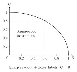
The same readout contrast $\eta$ permits different disturbance. For the square-root instrument, unread off-diagonal elements retain the factor $C=\sqrt{1-\eta^2}$; a sharp measurement followed by label noise fully removes them. At $\eta=3/5$, the first instrument retains $4/5$ of the initial coherence.

Same POVM, Different Instrument

The unsharp effects do not determine the backaction. The same $E_\pm$ can also arise from a sharp projective measurement followed by classical mislabeling.

For example, define

$$\mathcal I_+^{\mathrm{label}}(\rho) = \frac{1+\eta}{2}P_+\rho P_+ + \frac{1-\eta}{2}P_-\rho P_-,$$

and

$$\mathcal I_-^{\mathrm{label}}(\rho) = \frac{1-\eta}{2}P_+\rho P_+ + \frac{1+\eta}{2}P_-\rho P_-.$$

This instrument has the same effects $E_\pm$, because the probabilities are the same. But its nonselective channel is

$$\Phi_{\mathrm{label}}(\rho) = P_+\rho P_+ + P_-\rho P_-,$$

which fully dephases the $\sigma_z$ basis for every value of $\eta$. Even when $\eta$ is small and the reported label is almost random, the system was sharply measured before the label noise was applied.

Therefore “unsharp POVM” does not by itself mean “gentle measurement.” Gentleness is a property of the instrument.

Unsharp Versus Weak

The terms “unsharp” and “weak” overlap but are not identical.

An unsharp measurement has effects that do not perfectly distinguish the sharp alternatives. A weak measurement is usually a measurement regime in which each individual interaction gains little information and causes small disturbance, often as a step toward a repeated or continuous measurement.

The square-root instrument with small $\eta$ is weak in a common operational sense: each outcome only slightly biases the state and the nonselective dephasing is small:

$$\sqrt{1-\eta^2} \approx 1-\frac{\eta^2}{2} \qquad (\eta\ll1).$$

But a noisy-label instrument with the same small $\eta$ can be highly disturbing because it first performs a sharp measurement. Thus weak measurement requires assumptions about the instrument, not only the effects.

Finite-Resolution Pointers

Unsharpness also appears in continuous pointer models. In the von Neumann measurement model, different eigenvalues of $A$ shift a pointer wavepacket by different amounts. If the shifted packets overlap substantially, the pointer readout cannot distinguish the alternatives sharply.

A finite-resolution readout can be represented by effects such as

$$E_y = \int dx\,R(y|x)\,|x\rangle\langle x|,$$

Here $E_y$ is an effect density relative to $dy$, and $R(y|x)\ge0$ satisfies $\int R(y|x)\,dy=1$ for each $x$. The effect of a reported interval $B$ is $E(B)=\int_B E_y\,dy$, which obeys $0\le E(B)\le I$. A density $E_y$ itself need not be bounded above by $I$ and has units inverse to those of $y$. Broad response functions smear the sharp position question; they still do not uniquely specify the state update.

The von Neumann measurement model derives a Gaussian example from an explicit apparatus coupling.

Sequential Consequences

Unsharp measurements are useful in sequential experiments because they can extract partial information while leaving some coherence for later tests. For the square-root qubit instrument, a later $\sigma_x$ measurement after an unread unsharp $\sigma_z$ measurement has its contrast reduced by the factor $\sqrt{1-\eta^2}$ rather than erased completely.

This makes unsharp measurements central in:

• tests that balance information gain against invasiveness;
• continuous monitoring as a limit of many small updates;
• feedback protocols where the record is noisy but useful;
• measurement tomography, where one estimates detector effects and instruments;
• weak-value experiments, where weak coupling is followed by postselection.

The ordered-probability framework is Compatible, Incompatible, and Sequential Measurements.

Repeated readings need not repeat the label

For an input $|+z\rangle$, the square-root instrument preserves that state, yet each reading gives $-$ with probability $(1-\eta)/2$. Thus even an undisturbed eigenstate does not imply identical noisy reports. The projective repeatability rule is recovered only at $\eta=1$.

With fresh identical apparatuses, no intervening rotations, and a fixed $z$ eigenstate, successive labels are independent. For an unknown initial mixture, the labels become correlated after averaging over the possible eigenstate. Repeated readings progressively update that mixture’s probabilities rather than establishing a guaranteed answer from one reading.

Exercises

Positivity and Completeness

Show that

$$E_\pm = \frac{1}{2} \left( I\pm\eta\sigma_z \right)$$

defines a POVM for $0\le\eta\le1$.

Solution

The effects sum to

$$E_+ + E_- = \frac{1}{2}(I+\eta\sigma_z) + \frac{1}{2}(I-\eta\sigma_z) =I.$$

In the $\sigma_z$ basis, the eigenvalues of $E_+$ are $(1+\eta)/2$ and $(1-\eta)/2$, and the eigenvalues of $E_-$ are the same pair in the opposite order. These are nonnegative for $0\le\eta\le1$. Therefore the effects are positive and complete.

Bloch-Vector Probabilities

For

$$\rho = \frac{1}{2} \left( I+\mathbf r\cdot\boldsymbol\sigma \right),$$

derive $p(\pm)=(1\pm\eta r_z)/2$.

Solution

Use $\operatorname{Tr}\rho=1$, $\operatorname{Tr}(\rho\sigma_z)=r_z$, and

$$E_\pm = \frac{1}{2} \left( I\pm\eta\sigma_z \right).$$

Then

$$p(\pm) = \operatorname{Tr}(\rho E_\pm) = \frac{1}{2} \left[ \operatorname{Tr}\rho \pm \eta\operatorname{Tr}(\rho\sigma_z) \right] = \frac{1}{2}(1\pm\eta r_z).$$

Nonselective Dephasing Factor

Using the square-root operators $M_\pm=\sqrt{E_\pm}$, show that the off-diagonal matrix element $\rho_{01}$ is multiplied by $\sqrt{1-\eta^2}$.

Solution

Write

$$M_+ = aP_+ + bP_-, \qquad M_- = bP_+ + aP_-,$$

where

$$a=\sqrt{\frac{1+\eta}{2}}, \qquad b=\sqrt{\frac{1-\eta}{2}}.$$

The off-diagonal element in $M_+\rho M_+^\dagger$ is $ab\rho_{01}$, and the off-diagonal element in $M_-\rho M_-^\dagger$ is also $ab\rho_{01}$. Therefore the total factor is

$$2ab = 2\sqrt{ \frac{1+\eta}{2} \frac{1-\eta}{2} } = \sqrt{1-\eta^2}.$$

Same Effects, Different Disturbance

Compare the square-root instrument with the noisy-label instrument for the same effects $E_\pm$. What happens to $\rho_{01}$ when the outcome is ignored?

Solution

For the square-root instrument, the unread channel maps

$$\rho_{01} \longmapsto \sqrt{1-\eta^2}\,\rho_{01}.$$

For the noisy-label instrument, the unread channel is

$$\rho \longmapsto P_+\rho P_+ + P_-\rho P_-,$$

so

$$\rho_{01}\longmapsto0.$$

The effects, and therefore the outcome probabilities, are the same. The disturbance differs because the instruments are different.

References

• P. Busch, P. Lahti, and P. Mittelstaedt, The Quantum Theory of Measurement, second edition, Springer (1996). Publisher.
• P. Busch, P. Lahti, J.-P. Pellonpää, and K. Ylinen, Quantum Measurement, Springer (2016). Publisher.
• H. M. Wiseman and G. J. Milburn, Quantum Measurement and Control, Cambridge University Press (2010). Publisher.