Quantum Thermometry

Quantum thermometry is temperature estimation when the probe, sample, or measurement record must be described quantum mechanically. It includes simple equilibrium thermometers, nanoscale probes that disturb the sample, continuously monitored open systems, and nonequilibrium devices where the word “temperature” must be justified before it is estimated.

The central idea is statistical: temperature is inferred from data generated by a parameter-dependent quantum model. The model may be a Gibbs state, a thermal master equation, a noise spectrum, a relaxation curve, or a steady state of a probe. Thermometry is only as meaningful as that model.

There is no universal temperature operator. A thermometer is a physical procedure that maps an unknown thermal parameter to measurement outcomes, with uncertainty, backaction, calibration, and systematic error.

Equilibrium Thermometry

For a system with a temperature-independent Hamiltonian $H$ in equilibrium at temperature $T>0$, the Gibbs state is

$$\rho_T = \frac{e^{-\beta H}} {Z(T)}, \qquad \beta=\frac{1}{k_B T}, \qquad Z(T)=\operatorname{Tr}(e^{-\beta H}).$$

If a measurement with outcomes $x$ is described by POVM elements $E_x$, then the outcome probabilities are

$$p(x\mid T) = \operatorname{Tr}(E_x\rho_T).$$

This is now an ordinary parameter-estimation problem. The temperature dependence is encoded in the probability distribution $p(x\mid T)$.

The classical Fisher information for a chosen measurement is

$$\mathcal I_T = \sum_x p(x\mid T) \left[ \partial_T \ln p(x\mid T) \right]^2,$$

with the usual replacement by an integral for continuous outcomes. For $\nu$ independent repetitions and an unbiased estimator $\widehat T$, the Cramér–Rao bound is

$$\operatorname{Var}(\widehat T) \ge \frac{1}{\nu\,\mathcal I_T}.$$

See Fisher Information for the regularity and local unbiasedness conditions. Saturation is typically an asymptotic statement, not a guarantee for a small sample of rare events.

Quantum Fisher Information

The quantum Fisher information optimizes over measurements allowed by the quantum state family $\rho_T$. For an equilibrium Gibbs state with fixed Hamiltonian, the optimal measurement is energy measurement, because $\rho_T$ is diagonal in the energy eigenbasis for every $T$.

For temperature as the parameter,

$$F_Q(T) = \frac{\operatorname{Var}_{\rho_T}(H)} {k_B^2 T^4},$$

where

$$\operatorname{Var}_{\rho_T}(H) = \operatorname{Tr}(\rho_T H^2) - \left[ \operatorname{Tr}(\rho_T H) \right]^2 .$$

Equivalently, using the heat capacity

$$C(T) = \partial_T \operatorname{Tr}(\rho_T H),$$

one has

$$C(T) = \frac{\operatorname{Var}_{\rho_T}(H)} {k_B T^2}, \qquad F_Q(T) = \frac{C(T)} {k_B T^2}.$$

This relation is a useful anchor: equilibrium thermometric sensitivity is controlled by energy fluctuations, or equivalently by heat capacity. If the energy distribution barely changes with temperature, no measurement can estimate temperature sharply from that equilibrium state.

For inverse temperature $\beta$ as the parameter, the corresponding quantum Fisher information is especially simple:

$$F_Q(\beta) = \operatorname{Var}_{\rho_\beta}(H).$$

The temperature form follows by the chain rule because

$$\frac{d\beta}{dT} = - \frac{1}{k_B T^2}.$$

Qubit Thermometer

Consider a two-level probe with

$$H = \epsilon |e\rangle\langle e|, \qquad \epsilon\gt0.$$

In equilibrium,

$$p_e(T) = \frac{1} {1+e^{\beta\epsilon}}, \qquad p_g(T)=1-p_e(T).$$

An energy measurement is a Bernoulli experiment. The energy variance is

$$\operatorname{Var}(H) = \epsilon^2 p_e(1-p_e),$$

so the quantum Fisher information is

$$F_Q(T) = \frac{\epsilon^2} {k_B^2T^4} p_e(1-p_e).$$

It is helpful to write

$$x = \frac{\epsilon}{k_B T}.$$

Then

$$F_Q(T) = \frac{1}{T^2} \frac{x^2 e^x} {(1+e^x)^2} = \frac{1}{T^2} \frac{x^2} {4\cosh^2(x/2)}.$$

The sensitivity is poor when $x$ is very large because the excited state is almost never populated. It is also poor when $x$ is very small because the state is close to maximally mixed and changes slowly with $T$. The best gap is comparable to $k_BT$, with the dimensionless optimum determined by

$$x\tanh(x/2)=2.$$

Here the optimization varies the gap $\epsilon$ at a fixed target temperature $T$. Numerically this gives $x\approx2.4$. The main lesson is not the number; it is the matching principle. A good equilibrium thermometer has spectral features near the thermal energy scale.

Harmonic Oscillator Thermometer

For a harmonic oscillator,

$$H = \hbar\omega \left( a^\dagger a+\frac{1}{2} \right),$$

the equilibrium occupation is

$$\bar n(T) = \frac{1} {e^{\beta\hbar\omega}-1}.$$

The energy variance is

$$\operatorname{Var}(H) = (\hbar\omega)^2 \bar n(\bar n+1).$$

Therefore

$$F_Q(T) = \frac{(\hbar\omega)^2} {k_B^2T^4} \bar n(\bar n+1).$$

Unlike the qubit, an ideal oscillator has infinitely many levels. Its relative-temperature information is

$$T^2F_Q(T)=\frac{x^2}{4\sinh^2(x/2)}, \qquad x=\frac{\hbar\omega}{k_BT}.$$

At a fixed target temperature this increases toward $1$ as the gap decreases, rather than having a finite optimal gap. In the high-temperature limit $F_Q\to1/T^2$, so the best relative uncertainty per $\nu$ independent energy measurements approaches $1/\sqrt\nu$. A fixed gapped oscillator still loses sensitivity exponentially as $T\to0$. Practical low-frequency probes can have slow equilibration and limited readout resolution, constraints absent from this ideal state-based comparison.

Oscillators are common thermometric probes in optomechanics, ion traps, circuit resonators, and phononic systems. In practice, one often estimates temperature from sideband asymmetry, occupation number, quadrature noise, or relaxation dynamics rather than from an ideal projective energy measurement.

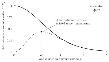
At fixed target temperature, the qubit has an optimal gap $\epsilon\simeq2.4k_BT$. An ideal oscillator instead approaches $T^2F_Q=1$ as its gap decreases. These curves describe independent equilibrium samples and ideal energy readout; they do not include equilibration time.

Probe Thermometry

In nanoscale thermometry, the object whose temperature is sought may be too small to measure directly. A probe is coupled to the sample, allowed to interact, and then measured. The model has the schematic form

$$\rho_P(T,t) = \Phi_T^t(\rho_P(0)),$$

where $\Phi_T^t$ is the probe dynamics induced by the sample and its environment.

Several regimes are common:

• equilibrium probe thermometry, where the probe thermalizes to a Gibbs state at the sample temperature;
• steady-state thermometry, where the probe reaches a nonequilibrium state that depends on $T$;
• transient thermometry, where information is extracted before equilibration;
• continuous thermometry, where a measurement record carries temperature information over time.

The best measurement time may be finite. If total laboratory time is the resource, compare information per preparation-and-measurement time, not only information per sample. Waiting longer can increase thermalization, but it can also reduce contrast, introduce decoherence, or heat the sample. The optimal protocol depends on the full open-system model, not only on the final equilibrium state.

Open-System Fisher Information

For a parameter-dependent master equation

$$\frac{d\rho_T}{dt} = \mathcal L_T(\rho_T),$$

temperature can enter through transition rates, noise spectra, detailed-balance ratios, or bath correlation functions. A measured record gives probabilities

$$p(\Gamma\mid T),$$

where $\Gamma$ may denote a trajectory, counting record, homodyne current, or final measurement outcome.

The Fisher information of the record is

$$\mathcal I_T^{\mathrm{rec}} = \sum_\Gamma p(\Gamma\mid T) \left[ \partial_T\ln p(\Gamma\mid T) \right]^2.$$

This is the natural language for continuously monitored thermometry. It connects to Stochastic Master Equations and quantum trajectories, where the information is distributed over a time series rather than a single final state.

For Markovian thermal models, detailed balance often makes temperature visible in excitation and relaxation rates. For a two-level transition of frequency $\omega$, one commonly has

$$\frac{\gamma_\uparrow} {\gamma_\downarrow} = e^{-\beta\hbar\omega}.$$

Estimating this ratio can estimate $T$, but only if the rates are actually thermal rates for the bath being probed.

Low-Temperature Limits

Low-temperature thermometry is hard because many finite systems become insensitive to $T$ as they approach the ground state. For a gapped probe with gap $\Delta$,

$$p_{\mathrm{exc}} \sim e^{-\Delta/(k_B T)}$$

at low temperature. The rare excited events carry information, but they occur exponentially infrequently.

This is related to the third law: cooling and certifying arbitrarily low temperatures become increasingly difficult under physical constraints. Gapless systems, dense spectra, impurity probes, critical systems, and many-body probes can improve scaling in some regimes, but they introduce other issues:

• equilibration may be slow;
• finite-size effects can dominate;
• the probe-sample coupling can disturb the sample;
• critical parameters may be uncertain;
• the relevant temperature may vary spatially.

Strong claims about low-temperature precision should therefore include both statistical and systematic uncertainties.

Critical and Many-Body Thermometry

Because equilibrium thermometric sensitivity is tied to heat capacity, many-body systems near phase transitions can be highly sensitive to temperature. Formally, large energy fluctuations can produce large $F_Q(T)$.

This observation is useful but not automatic. A realistic thermometer must still answer:

• how the probe equilibrates;
• which observable is measured;
• how close the system can be brought to criticality;
• whether finite-size rounding controls the signal;
• whether the relaxation time is compatible with the experiment;
• whether unknown Hamiltonian parameters mimic temperature changes.

Critical thermometry is therefore a tradeoff between enhanced susceptibility and model fragility.

Effective Temperatures

Open-system physics often uses effective temperatures. Examples include:

• a transition temperature inferred from a rate ratio;
• a noise temperature inferred from a spectrum;
• a fluctuation-dissipation temperature in a near-equilibrium regime;
• a local temperature assigned to a small subsystem;
• a mode temperature of a nonequilibrium bosonic field.

These quantities can be useful, but they need not agree with one another. A nonequilibrium environment may look thermal to one transition frequency and nonthermal to another. A squeezed reservoir can mimic a high occupation number while still containing phase-sensitive resources. A driven steady state can have a fitted temperature without being a Gibbs state.

The safest question is: which operational measurement defines this temperature, and over what frequency, timescale, and coupling regime is the definition valid? See Fluctuation–Dissipation Relation and Noise Spectra.

Backaction and Calibration

A thermometer is not passive by default. Coupling a probe to a small sample can exchange heat, change the sample’s state, broaden levels, or introduce extra noise. Repeated measurements can add heating. Feedback used to stabilize the probe can also become part of the thermodynamic accounting.

The practical error budget has two layers:

• statistical uncertainty, bounded locally by Fisher information;
• systematic uncertainty, caused by model mismatch, calibration drift, unknown coupling, finite sample heat capacity, and nonequilibrium effects.

Increasing Fisher information does not remove systematic error. For a concrete identifiability problem, the equilibrium qubit populations depend only on $x=\epsilon/(k_BT)$. If both $\epsilon$ and $T$ are unknown, population measurements alone determine their ratio, not either separately. The two-parameter Fisher matrix is singular. An independent gap calibration or another observable is required before the one-parameter temperature bound applies.

Exercises

Gibbs-State Fisher Information

For a finite-dimensional Gibbs state

$$\rho_T = \frac{e^{-\beta H}}{Z}, \qquad \beta=\frac{1}{k_BT},$$

show that the quantum Fisher information for estimating $T$ is

$$F_Q(T) = \frac{\operatorname{Var}_{\rho_T}(H)} {k_B^2T^4}.$$

Solution

Because $\rho_T$ is diagonal in the energy eigenbasis for every $T$, the optimal measurement is energy measurement. Let

$$p_n = \frac{e^{-\beta E_n}}{Z}.$$

Then

$$\partial_T\ln p_n = - E_n\partial_T\beta - \partial_T\ln Z.$$

Since

$$\partial_T\beta = - \frac{1}{k_BT^2}$$

and

$$\partial_T\ln Z = \frac{\langle H\rangle} {k_BT^2},$$

one obtains

$$\partial_T\ln p_n = \frac{E_n-\langle H\rangle} {k_BT^2}.$$

The Fisher information is therefore

$$F_Q(T) = \sum_n p_n \frac{(E_n-\langle H\rangle)^2} {k_B^2T^4} = \frac{\operatorname{Var}_{\rho_T}(H)} {k_B^2T^4}.$$

Qubit Optimum Condition

For the qubit thermometer, show that maximizing

$$f(x) = \frac{x^2} {4\cosh^2(x/2)}$$

over $x\gt0$ at fixed target temperature (varying the probe gap) gives

$$x\tanh(x/2)=2.$$

Solution

It is easiest to differentiate the logarithm:

$$\ln f(x) = 2\ln x-\ln4-2\ln\cosh(x/2).$$

Thus

$$\frac{d}{dx}\ln f(x) = \frac{2}{x} - \tanh(x/2).$$

At an interior maximum this derivative vanishes, so

$$\frac{2}{x} = \tanh(x/2),$$

or

$$x\tanh(x/2)=2.$$

Heat Capacity Relation

Show that for a canonical state with fixed Hamiltonian,

$$C(T) = \frac{\operatorname{Var}_{\rho_T}(H)} {k_B T^2}.$$

Solution

The mean energy is

$$\langle H\rangle = - \partial_\beta \ln Z.$$

Differentiating with respect to $\beta$ gives

$$\partial_\beta \langle H\rangle = - \partial_\beta^2\ln Z = - \operatorname{Var}_{\rho_T}(H).$$

Since

$$\frac{d\beta}{dT} = - \frac{1}{k_BT^2},$$

the heat capacity is

$$C(T) = \frac{d\langle H\rangle}{dT} = \partial_\beta\langle H\rangle \frac{d\beta}{dT} = \frac{\operatorname{Var}_{\rho_T}(H)} {k_BT^2}.$$

Effective Temperature Warning

A two-level probe coupled to a nonequilibrium environment has measured transition rates satisfying

$$\frac{\gamma_\uparrow}{\gamma_\downarrow} = e^{-\hbar\omega/(k_BT_{\mathrm{eff}})}.$$

Give two reasons why $T_{\mathrm{eff}}$ need not be a thermodynamic temperature of the environment.

Solution

First, the ratio probes the environment only at one transition frequency $\omega$. A nonequilibrium spectrum can mimic a thermal ratio at that frequency while failing detailed balance at other frequencies.

Second, the environment may contain additional resources such as driving, squeezing, chemical bias, or mode selectivity. These can alter transition rates without being equivalent to a Gibbs reservoir. The inferred $T_{\mathrm{eff}}$ is therefore an operational transition temperature, not automatically a full thermodynamic temperature.

References

• F. Binder, L. A. Correa, C. Gogolin, J. Anders, and G. Adesso, eds., Thermodynamics in the Quantum Regime: Fundamental Aspects and New Directions, Springer (2018).
• S. Campbell, M. Mehboudi, G. De Chiara, and M. Paternostro, “Global and local thermometry schemes in coupled quantum systems,” New Journal of Physics 19, 103003 (2017).
• L. A. Correa, M. Mehboudi, G. Adesso, and A. Sanpera, “Individual quantum probes for optimal thermometry,” Physical Review Letters 114, 220405 (2015). arXiv:1411.2437.
• A. De Pasquale, D. Rossini, R. Fazio, and V. Giovannetti, “Local quantum thermal susceptibility,” Nature Communications 7, 12782 (2016).
• C. W. Helstrom, Quantum Detection and Estimation Theory, Academic Press (1976).
• M. Mehboudi, A. Sanpera, and L. A. Correa, “Thermometry in the quantum regime: Recent theoretical progress,” Journal of Physics A: Mathematical and Theoretical 52, 303001 (2019).
• M. G. A. Paris, “Quantum estimation for quantum technology,” International Journal of Quantum Information 7, 125-137 (2009).