Non-Markovian Toy Models

An atom can transfer an excitation into a single mode and later receive it back. Evolving the atom and mode together gives a simple exact example of reduced dynamics with memory. This calculation checks a partial trace, distinguishes population revival from full state revival, and compares two trace-distance curves.

Helpful background. Reduced dynamics explains the joint-state construction. Information backflow explains what an increase of trace distance tests. The example uses Python 3 and NumPy.

Resonant exchange with a vacuum mode

Use the resonant Jaynes–Cummings interaction in its interaction picture,

$$H_I=\hbar g(\sigma_+\otimes a+\sigma_-\otimes a^\dagger), \qquad \sigma_-=|g\rangle\langle e|,$$

with real $g>0$ and an initially uncorrelated vacuum mode. This is an exact calculation within this rotating-wave model, not an exact solution of the full atom–field Hamiltonian. The total excitation number is conserved. Starting with at most one excitation therefore requires only mode states $|0\rangle$ and $|1\rangle$.

In the coupled subspace,

$$|e,0\rangle\longmapsto\cos(gt)|e,0\rangle-i\sin(gt)|g,1\rangle, \qquad |g,0\rangle\longmapsto|g,0\rangle.$$

Use system basis $(|g\rangle,|e\rangle)$ and system-first tensor order. For an arbitrary initial qubit state the reduced channel has

$$K_0(t)=\begin{pmatrix}1&0\\0&\cos(gt)\end{pmatrix}, \qquad K_1(t)=\begin{pmatrix}0&\sin(gt)\\0&0\end{pmatrix}.$$

In particular, $p_e(t)=\cos^2(gt)p_e(0)$ and $\rho_{ge}(t)=\cos(gt)\rho_{ge}(0)$. Keep the sign of the cosine: replacing it by $\sqrt{\cos^2(gt)}$ gives incorrect coherences after the first zero.

Calculate joint evolution and trace out the mode

For a Hermitian Hamiltonian, eigh gives an orthonormal eigenbasis, so multiplying its eigenvectors by $e^{-iE_nt}$ constructs the unitary without an ODE solver. The code repeats the calculation with mode dimensions two and three; both give the same answer in the populated excitation sectors.

import numpy as np

sm = np.array([[0, 1], [0, 0]], dtype=complex)
rho_y = np.array([[0.5, -0.5j], [0.5j, 0.5]])
rho_e = np.diag([0.0, 1.0])
rho_g = np.diag([1.0, 0.0])
g = 1.0

def reduced(rho, t, modes):
    a = np.diag(np.sqrt(np.arange(1, modes)), 1)
    H = g*(np.kron(sm.conj().T, a)+np.kron(sm, a.conj().T))
    E, V = np.linalg.eigh(H)
    U = (V*np.exp(-1j*E*t))@V.conj().T
    vacuum = np.zeros((modes, modes))
    vacuum[0, 0] = 1
    joint = U@np.kron(rho, vacuum)@U.conj().T
    return np.einsum('iaja->ij', joint.reshape(2, modes, 2, modes))

def analytic(rho, t):
    K0 = np.diag([1, np.cos(g*t)])
    K1 = np.array([[0, np.sin(g*t)], [0, 0]])
    return K0@rho@K0.conj().T+K1@rho@K1.conj().T

def distance(A, B):
    delta = A-B
    assert np.linalg.norm(delta-delta.conj().T) < 1e-12
    return np.abs(np.linalg.eigvalsh(delta)).sum()/2

assert np.allclose(reduced(rho_y, 0, 3), rho_y)
for t in [0, np.pi/4, np.pi/2, 3*np.pi/4, np.pi, 2*np.pi]:
    out = reduced(rho_y, t, 2)
    assert np.allclose(out, reduced(rho_y, t, 3))
    assert np.allclose(out, analytic(rho_y, t))
    assert np.linalg.eigvalsh(out).min() >= -1e-12
    D = distance(reduced(rho_e, t, 2), reduced(rho_g, t, 2))
    assert np.isclose(D, np.cos(g*t)**2)
    print('gt:', g*t, 'D(e,g):', D, 'imag coherence:', out[0, 1].imag)

Z = np.diag([1, -1])
assert np.allclose(reduced(rho_y, np.pi/g, 2), Z@rho_y@Z)
assert not np.allclose(reduced(rho_y, np.pi/g, 2), rho_y)
assert np.allclose(reduced(rho_y, 2*np.pi/g, 2), rho_y)

# A finite oscillator never has [a, a-dagger] = I exactly.
modes = 3
a = np.diag(np.sqrt(np.arange(1, modes)), 1)
commutator = a@a.conj().T-a.conj().T@a
assert np.allclose(commutator, np.diag([1, 1, -2]))

At $gt=\pi/2$, both initially ground and initially excited qubits end in the ground state, giving trace distance zero. At $gt=\pi$ their distinguishability returns to one. No channel acting only on their identical intermediate reduced states could separate them again. This directly rules out a completely positive divisible description across that interval, without trying to invert the singular intermediate map.

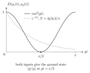
For the excited/ground input pair, the vacuum-mode model gives $D(t)=\cos^2(gt)$. Both reduced states become $|g\rangle\langle g|$ at $gt=\pi/2$, then separate again. The dashed exponential uses $\Gamma=4g\ln2/\pi$ to match the first half-population time, as explained below. It is a comparison curve, not a bath-derived approximation to the isolated mode.

What the comparison tells you

For a zero-temperature amplitude-damping semigroup, the same pair has $D_M(t)=e^{-\Gamma t}$. One transparent comparison is $\Gamma=4g\log2/\pi$, which matches the first half-population time $t=\pi/(4g)$. It does not match the initial slope: the exact population starts as $1-g^2t^2+O(t^4)$, whereas the exponential starts as $1-\Gamma t+O(t^2)$.

Each exact map from time zero is completely positive and trace preserving. A revival violates contraction for a putative channel between the intermediate times, not contraction from the initial states. Also, a single-pair calculation detects backflow here but does not optimize a non-Markovianity measure over all input pairs. The equatorial pair $|+\rangle,|-\rangle$ has $D(t)=|\cos(gt)|$, a different curve with the same zeros and revival times.

Finite mode truncation does not preserve the oscillator commutator: with $d$ retained number states, $[a,a^\dagger]=I-d|d-1\rangle\langle d-1|$. Nevertheless, the two-state truncation is exact on this model’s dynamically accessible zero- and one-excitation sectors. A drive or finite-temperature initial mode can populate more sectors and requires a new cutoff-convergence check.

Add a lossy mode only after the exact check

An enlarged-system model may include $\kappa\mathcal D[a]$, where $\kappa$ is the mode’s population decay rate. At resonance in the vacuum one-excitation problem, the qubit amplitude obeys

$$\ddot G+\frac\kappa2\dot G+g^2G=0, \qquad G(0)=1,\quad\dot G(0)=0.$$

Oscillatory amplitudes occur for $g>\kappa/4$. In the strongly damped limit $\kappa\gg g$, eliminating the rapidly decaying mode gives qubit amplitude decay $2g^2/\kappa$ and population decay $4g^2/\kappa$. Distinguish these two rates. Matching such an enlarged model to a particular bath requires the spectral assumptions described in pseudomode methods; simply adding a mode is not a universal reservoir model.

Exercises

Population versus state revival. Why is $t=\pi/g$ not a full revival for an arbitrary qubit state?

Solution

At that time $K_0=Z$ and $K_1=0$, so the channel is $\rho\mapsto Z\rho Z$. Populations return, but coherences change sign. The full channel first returns to the identity at $2\pi/g$.

A different input pair. Derive the trace distance for $|+\rangle$ and $|-\rangle$.

Solution

Their density-matrix difference is $X$. The channel maps it to $\cos(gt)X$, whose eigenvalues are $\pm\cos(gt)$. Half the trace norm is $|\cos(gt)|$.

No inverse at the reset time. Why does $\Phi_t\Phi_s^{-1}$ fail at $gs=\pi/2$?

Solution

$\Phi_s$ sends every trace-one input to the ground state, so it is not invertible as a linear map on operators. The impossibility of subsequent separation of identical inputs proves the lack of divisibility directly.

Eliminate a fast mode. Derive the slow population-decay rate from $\dot G=-igb$ and $\dot b=-igG-(\kappa/2)b$.

Solution

When $\kappa\gg g$ and after the initial fast transient, set $\dot b\simeq0$, obtaining $b\simeq-2igG/\kappa$. Then $\dot G\simeq-2g^2G/\kappa$, so $|G|^2$ decays at rate $4g^2/\kappa$.

References

• H.-P. Breuer, E.-M. Laine, and J. Piilo, “Measure for the degree of non-Markovian behavior of quantum processes in open systems,” Physical Review Letters 103, 210401 (2009). doi:10.1103/PhysRevLett.103.210401.
• H.-P. Breuer and F. Petruccione, The Theory of Open Quantum Systems, Oxford University Press (2002).
• I. de Vega and D. Alonso, “Dynamics of non-Markovian open quantum systems,” Reviews of Modern Physics 89, 015001 (2017). doi:10.1103/RevModPhys.89.015001.
• B. M. Garraway, “Nonperturbative decay of an atomic system in a cavity,” Physical Review A 55, 2290–2303 (1997). doi:10.1103/PhysRevA.55.2290.