Pseudomode Methods

Pseudomode methods replace part of a structured environment by one or more explicit damped modes. The enlarged system evolves with an ordinary Markovian master equation, while the original smaller system can show non-Markovian memory after those modes are traced out.

The schematic idea is:

structured reservoir = pseudomode(s) + broadband residual bath

This is especially useful when the environmental spectrum has narrow Lorentzian features, cavity-like resonances, or a small number of poles that dominate the bath correlation function. The method does not deny memory. It relocates memory from an implicit bath kernel into explicit auxiliary degrees of freedom.

For the broad terminology of memory effects, see Non-Markovian Dynamics. For the integral-equation language that pseudomodes often simplify, see Memory Kernels.

A System Coupled to a Damped Mode

Start with a system operator $L$ coupled to a bosonic environment in a rotating-wave form,

$$H = H_S + \sum_k\hbar\omega_k b_k^\dagger b_k + \hbar\sum_k \left( g_k L^\dagger b_k + g_k^* L b_k^\dagger \right).$$

The environment is summarized by a spectral density such as

$$J(\omega) = \sum_k |g_k|^2\delta(\omega-\omega_k).$$

If the bath is initially in vacuum, the relevant correlation function has the form

$$C(t) = \int d\omega\, J(\omega)e^{-i(\omega-\omega_0)t}, \qquad t\ge0,$$

Here $g_k$ and $g$ have units of angular frequency, $J$ has units of inverse time, and $C$ has units of inverse time squared; $L$ is dimensionless. The displayed integral uses the interaction picture at $\omega_0$. A featureless broadband $J(\omega)$ gives a short correlation time and often leads to a Markovian dissipator. A structured $J(\omega)$ gives a longer-lived $C(t)$ and hence memory.

The pseudomode strategy is to approximate or exactly represent this correlation by damped auxiliary modes. For one pseudomode $a$, the enlarged density matrix $\varrho$ obeys

$$\frac{d\varrho}{dt} = - \frac{i}{\hbar} [H_{\mathrm{aug}},\varrho] + \kappa\mathcal D[a]\varrho,$$

with

$$H_{\mathrm{aug}} = H_S + \hbar\omega_c a^\dagger a + \hbar \left( g L^\dagger a + g^* L a^\dagger \right).$$

The residual bath damping the pseudomode is Markovian. The original system state is recovered by

$$\rho_S(t) = \operatorname{Tr}_a\varrho(t).$$

The enlarged $S+a$ dynamics is time-local and Lindblad. The reduced $S$ dynamics need not be CP-divisible or time-local with nonnegative rates.

Lorentzian Spectrum

Choose the mode phase so that $g\ge0$ is real. The standard single-pseudomode example is a Lorentzian spectral density centered at $\omega_c$:

$$J(\omega) = \frac{1}{2\pi} \frac{g^2\kappa} {(\omega-\omega_c)^2+(\kappa/2)^2}.$$

In a rotating frame at $\omega_0$, define the detuning

$$\Delta=\omega_c-\omega_0.$$

Extending the detuning integral to the whole real line gives

$$C(t) = g^2 e^{-(\kappa/2+i\Delta)t}, \qquad t\ge0.$$

This is exactly the correlation of the stated damped-mode model, with amplitude-correlation time $2/\kappa$. For a physical bath restricted to positive laboratory frequencies, extending the integral below zero is an approximation, usually useful near a narrow resonance far above the lower frequency edge. The extended Lorentzian does not reproduce the threshold or long-time tails of every physical reservoir.

The Lorentzian example is not just convenient algebra. It captures a real physical situation: a system coupled strongly to a leaky cavity-like resonance, which in turn leaks into a broad continuum.

Memory from Tracing the Pseudomode

Consider a two-level system coupled to one pseudomode in the single-excitation sector. Let $c_e(t)$ be the amplitude for the excited system and empty pseudomode, and let $c_p(t)$ be the amplitude for the ground system and one pseudomode excitation. For real $g$, in a rotating frame,

$$\dot c_e(t) = -ig c_p(t),$$

and

$$\dot c_p(t) = - \left( \frac{\kappa}{2}+i\Delta \right)c_p(t) -ig c_e(t).$$

For $c_p(0)=0$, the second equation gives

$$c_p(t) = -ig \int_0^t ds\, e^{-(\kappa/2+i\Delta)(t-s)} c_e(s).$$

Substituting into the first equation yields

$$\dot c_e(t) = - g^2 \int_0^t ds\, e^{-(\kappa/2+i\Delta)(t-s)} c_e(s).$$

The enlarged model is Markovian, but the eliminated amplitude has an explicit memory kernel. This is the practical essence of the method.

Excitation Return on Resonance

At $\Delta=0$, differentiate the equation for $c_e$ once and eliminate $c_p$:

$$\ddot c_e+\frac{\kappa}{2}\dot c_e+g^2c_e=0.$$

For an initially excited qubit and vacuum mode, $c_e(0)=1$ and $\dot c_e(0)=0$. When $g>\kappa/4$, write $\Omega_R=\sqrt{g^2-\kappa^2/16}$ to obtain

$$c_e(t)=e^{-\kappa t/4} \left[\cos(\Omega_Rt)+\frac{\kappa}{4\Omega_R}\sin(\Omega_Rt)\right].$$

The qubit population is $p_e(t)=|c_e(t)|^2$. These amplitudes describe the unnormalized no-emission component; after an emission, the qubit and mode are in their ground state, so the same expression gives the unconditional excited population. If $g<\kappa/4$, replace the trigonometric functions by their hyperbolic continuation. At the boundary, $c_e(t)=e^{-\kappa t/4}(1+\kappa t/4)$.

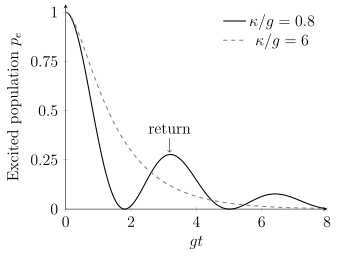
Exact resonant populations for $g>0$. For $\kappa/g=0.8$, excitation returns from the mode after the first minimum. For $\kappa/g=6$, loss suppresses that exchange. Both curves start with zero slope, unlike a simple exponential approximation valid after the mode’s short transient.

Markov Limit

When the pseudomode decays much faster than the system exchanges excitation with it,

$$\kappa\gg g,$$

the kernel is sharply concentrated near $s=t$. On resonance, one approximates

$$\int_0^t ds\, e^{-\kappa(t-s)/2} c_e(s) \approx \frac{2}{\kappa}c_e(t).$$

The amplitude then obeys

$$\dot c_e(t) \approx - \frac{2g^2}{\kappa}c_e(t).$$

The excited-state population decays at the approximate rate

$$\Gamma \approx \frac{4g^2}{\kappa}.$$

This is the same bad-cavity scaling that appears in many effective-decay and reservoir-engineering arguments. The important lesson is the hierarchy: a rapidly reset pseudomode can be eliminated into a Markovian decay channel, while a slowly reset pseudomode must remain explicit.

Multiple Pseudomodes

Many structured correlations are well approximated by sums of exponentials:

$$C(t) \approx \sum_{j=1}^M |g_j|^2 e^{-(\kappa_j/2+i\Delta_j)t}.$$

A natural enlarged model uses $M$ damped modes,

$$H_{\mathrm{aug}} = H_S + \sum_j\hbar\omega_j a_j^\dagger a_j + \hbar\sum_j \left( g_j L^\dagger a_j + g_j^* L a_j^\dagger \right),$$

with dissipators

$$\sum_j \kappa_j\mathcal D[a_j]\varrho.$$

This model produces a correlation function with the same exponential components when the pseudomodes are initially in vacuum and independently damped.

More general spectral densities may require coupled pseudomodes, correlated damping, finite-temperature residual baths, or a different mapping. A numerical sum of exponentials should be checked as a physical open-system dilation, not only as a curve fit.

If the goal is to use the exponential correlation expansion directly rather than interpret each term as a damped mode, see Hierarchical Equations of Motion.

Relation to Cavity and Input-Output Models

A pseudomode often looks like a lossy cavity mode. In an optical or microwave implementation, that may be literally true: the system couples to a resonator, and the resonator couples to a transmission line. Then the enlarged Lindblad model is also an Input–Output Theory model.

In other settings, the pseudomode is an effective mathematical degree of freedom. It represents a pole of the environmental response rather than a directly addressable oscillator. This distinction matters experimentally, but the reduced dynamics can be the same within the modeled sector.

Pseudomode methods are closely related in spirit to moving the system-bath boundary. A strongly coupled environmental feature becomes part of the enlarged system; the remaining environment is treated as shorter-memory and more nearly Markovian. Reaction-Coordinate Mapping develops this boundary-change idea for collective bath coordinates, and System-Bath Hamiltonians discusses the modeling choice more generally.

What the Method Guarantees

If the enlarged equation is a valid Lindblad equation, then the map on $S+a_1+\cdots+a_M$ is completely positive and trace preserving. Tracing out the pseudomodes gives a completely positive trace-preserving map for the original system at each final time:

$$\rho_S(t) = \operatorname{Tr}_{a_1\cdots a_M} \Phi_t^{\mathrm{aug}} \left( \rho_S(0)\otimes\rho_{\mathrm{pm}}(0) \right).$$

This final-time physicality is valuable. It is one reason pseudomode embeddings are safer than arbitrary fitted memory kernels.

However, it does not imply that the reduced system evolution is Markovian. Intermediate reduced maps can fail CP divisibility, and trace distance can temporarily increase for some pairs of states. Those are not failures of the pseudomode construction; they are the memory effects the construction is designed to represent.

Finite Temperature and Detailed Balance

The simplest pseudomode model assumes a vacuum residual bath:

$$\kappa\mathcal D[a]\varrho.$$

At finite temperature one often needs

$$\kappa(\bar n+1)\mathcal D[a]\varrho + \kappa\bar n\,\mathcal D[a^\dagger]\varrho,$$

or a more careful microscopic model. If the original environment is thermal, the enlarged model should reproduce the relevant thermal correlation functions and detailed-balance relations. A damped mode at the wrong occupation can give the right linewidth and the wrong steady state. A single constant $\bar n$ across a finite linewidth also need not satisfy the exact thermal frequency relation throughout that linewidth; treating it as a thermal reservoir requires the corresponding narrow-band or weak-coupling approximation.

For thermal-rate consistency, compare with Thermal Master Equations and Noise Spectra.

Numerical Workflow

For a finite-dimensional system coupled to truncated pseudomodes:

1. Choose the spectral feature or bath correlation to reproduce.
2. Fit or derive pseudomode parameters $g_j$, $\omega_j$, and $\kappa_j$.
3. Build the enlarged Hamiltonian and Lindblad dissipators.
4. Choose a Fock cutoff for each pseudomode and test convergence.
5. Evolve the enlarged density matrix.
6. Trace out pseudomodes to obtain system observables.
7. Compare the reproduced $C(t)$ or $J(\omega)$ with the intended environment.
8. Test reduced non-Markovian diagnostics only after specifying the system-only map.

The linear-algebra checks in Solving Lindblad Equations apply to the enlarged Liouvillian. The reduced system may not have a time-independent Liouvillian of its own.

When One Mode Is Insufficient

A single Lorentzian gives one exponential correlation. Band edges, algebraic tails, sub-Ohmic spectra, and finite spin baths generally require more modes or another method. Bosonic mode truncations must also be checked at the strongest drive and highest temperature being modeled; low-excitation convergence does not establish convergence in those regimes.

Exercises

Eliminate One Pseudomode

Starting from

$$\dot c_e(t) = -ig c_p(t), \qquad \dot c_p(t) = - \left( \frac{\kappa}{2}+i\Delta \right)c_p(t) -ig c_e(t),$$

with $c_p(0)=0$, derive the memory equation for $c_e(t)$.

Solution

The pseudomode equation is linear. Multiply by the integrating factor

$$e^{(\kappa/2+i\Delta)t}.$$

Then

$$\frac{d}{dt} \left[ e^{(\kappa/2+i\Delta)t}c_p(t) \right] = -ig e^{(\kappa/2+i\Delta)t}c_e(t).$$

Integrating from $0$ to $t$ and using $c_p(0)=0$ gives

$$c_p(t) = -ig \int_0^t ds\, e^{-(\kappa/2+i\Delta)(t-s)} c_e(s).$$

Substituting into $\dot c_e=-igc_p$ gives

$$\dot c_e(t) = - g^2 \int_0^t ds\, e^{-(\kappa/2+i\Delta)(t-s)} c_e(s).$$

Bad-Cavity Limit

On resonance, use the approximation $\kappa\gg g$ to find the population-decay rate implied by the pseudomode memory kernel.

Solution

When $\kappa$ is large, $c_e(s)$ changes slowly over the kernel width. Approximate $c_e(s)\approx c_e(t)$ in

$$\dot c_e(t) = - g^2 \int_0^t ds\, e^{-\kappa(t-s)/2} c_e(s).$$

For times large compared with $\kappa^{-1}$,

$$\int_0^t ds\, e^{-\kappa(t-s)/2} \approx \int_0^\infty d\tau\, e^{-\kappa\tau/2} = \frac{2}{\kappa}.$$

Thus

$$\dot c_e(t) \approx - \frac{2g^2}{\kappa}c_e(t).$$

The amplitude decay rate is $2g^2/\kappa$, so the population decay rate is

$$\Gamma \approx \frac{4g^2}{\kappa}.$$

Damped-Mode Correlation

For a vacuum damped mode with equation

$$\dot\varrho = - i[\Delta a^\dagger a,\varrho] + \kappa\mathcal D[a]\varrho,$$

show that its vacuum correlation is proportional to

$$e^{-(\kappa/2+i\Delta)t}.$$

Solution

The adjoint Markov semigroup acting on the mode observable gives

$$\frac{d}{dt}a(t) = - \left( \frac{\kappa}{2}+i\Delta \right)a(t).$$

Therefore

$$a(t) = e^{-(\kappa/2+i\Delta)t}a(0).$$

For the vacuum state,

$$\langle a(t)a^\dagger(0)\rangle = e^{-(\kappa/2+i\Delta)t} \langle a(0)a^\dagger(0)\rangle = e^{-(\kappa/2+i\Delta)t}.$$

The two-time expression follows from quantum regression for this Markov mode. The full Heisenberg–Langevin operator additionally contains input noise; dropping that noise would not preserve its equal-time commutator. Multiplying the correlation by $g^2$ gives the environmental correlation component.

Reduced Versus Enlarged Divisibility

Explain why a Lindblad equation for $S+a$ does not automatically imply CP divisibility for the reduced system $S$.

Solution

The enlarged evolution has CPTP maps

$$\Phi_t^{S+a} = e^{t\mathcal L_{\mathrm{aug}}}.$$

The reduced state is

$$\rho_S(t) = \operatorname{Tr}_a \Phi_t^{S+a} \left( \rho_S(0)\otimes\rho_a(0) \right).$$

This gives a CPTP map from the initial system state to the final system state. But after an intermediate time $s$, the state of $S$ is generally correlated with the pseudomode. The future state of $S$ depends on those hidden correlations and on the pseudomode state, not only on $\rho_S(s)$. Therefore an intermediate map acting only on $\rho_S(s)$ need not be CPTP or even well defined for all reduced states.

References

• H.-P. Breuer and F. Petruccione, The Theory of Open Quantum Systems, Oxford University Press (2002).
• H.-P. Breuer, E.-M. Laine, J. Piilo, and B. Vacchini, “Colloquium: Non-Markovian dynamics in open quantum systems,” Reviews of Modern Physics 88, 021002 (2016).
• B. J. Dalton, S. M. Barnett, and B. M. Garraway, “Theory of pseudomodes in quantum optical processes,” Physical Review A 64, 053813 (2001).
• I. de Vega and D. Alonso, “Dynamics of non-Markovian open quantum systems,” Reviews of Modern Physics 89, 015001 (2017).
• B. M. Garraway, “Decay of an atom coupled strongly to a reservoir,” Physical Review A 55, 4636-4639 (1997).
• B. M. Garraway, “Nonperturbative decay of an atomic system in a cavity,” Physical Review A 55, 2290-2303 (1997).
• G. Pleasance, B. M. Garraway, and F. Petruccione, “Generalized theory of pseudomodes for exact descriptions of non-Markovian quantum processes,” Physical Review Research 2, 043058 (2020).