Reduced Dynamics

Reduced dynamics is the time evolution assigned to a subsystem after the degrees of freedom outside that subsystem are ignored.

The central formula is:

$$\rho_S(t) = \operatorname{Tr}_E \left[ U_{SE}(t,t_0)\rho_{SE}(t_0)U_{SE}^\dagger(t,t_0) \right].$$

The total system $S+E$ may evolve unitarily. The subsystem $S$ can still evolve nonunitarily because information, coherence, and energy can move into correlations with $E$.

Helpful background. The partial trace extracts subsystem predictions; complete positivity describes maps that remain physical when a reference system is retained.

Exact Reduced State

Let the total Hilbert space be

$$\mathcal H_{SE} = \mathcal H_S\otimes\mathcal H_E.$$

If the total state at time $t$ is $\rho_{SE}(t)$, then the reduced state of $S$ is

$$\rho_S(t) = \operatorname{Tr}_E\rho_{SE}(t).$$

If the total evolution is unitary,

$$\rho_{SE}(t) = U_{SE}(t,t_0)\rho_{SE}(t_0)U_{SE}^\dagger(t,t_0).$$

Combining these equations gives the exact reduced dynamics formula:

$$\rho_S(t) = \operatorname{Tr}_E \left[ U_{SE}(t,t_0)\rho_{SE}(t_0)U_{SE}^\dagger(t,t_0) \right].$$

This equation is always true when the total unitary model and initial total state are specified. It is not yet a closed equation for $\rho_S(t)$ alone.

Factorized Initial State

A common starting assumption is an initially uncorrelated system-environment state:

$$\rho_{SE}(t_0) = \rho_S(t_0)\otimes\eta_E,$$

where $\eta_E$ is a fixed environment reference state, independent of the input $\rho_S(t_0)$, and the same joint unitary is used for every input.

Then the reduced state can be written as a map on the initial system state:

$$\rho_S(t) = \Phi_{t,t_0}\bigl(\rho_S(t_0)\bigr),$$

with

$$\Phi_{t,t_0}(\rho) = \operatorname{Tr}_E \left[ U_{SE}(t,t_0)(\rho\otimes\eta_E) U_{SE}^\dagger(t,t_0) \right].$$

This map is completely positive and trace preserving. It is a quantum channel.

The factorized-state assumption is not a theorem. It is a modeling assumption that can fail when the system and environment are already correlated before the time interval of interest.

Kraus Form from the Environment

The channel form can be made explicit. Diagonalize the environment reference state:

$$\eta_E = \sum_r q_r |r\rangle\langle r|, \qquad q_r\ge0, \qquad \sum_r q_r=1.$$

Choose an orthonormal environment basis $\{|\mu\rangle\}$ for the final partial trace. Define operators on the system by

$$K_{\mu r}(t,t_0) = \sqrt{q_r}\, \langle\mu| U_{SE}(t,t_0) |r\rangle.$$

The bracket is taken only over the environment Hilbert space, leaving a system operator. Then

$$\Phi_{t,t_0}(\rho) = \sum_{\mu,r} K_{\mu r}(t,t_0)\rho K_{\mu r}^\dagger(t,t_0).$$

The trace-preserving condition follows from unitarity:

$$\sum_{\mu,r} K_{\mu r}^\dagger K_{\mu r} = I_S.$$

This derivation is one of the cleanest ways to see why reduced dynamics is described by completely positive maps when the initial state is factorized.

What Nonunitarity Means

The reduced map $\Phi_{t,t_0}$ usually does not have the form

$$\rho_S \longmapsto U_S\rho_SU_S^\dagger.$$

It may shrink or translate Bloch vectors, suppress off-diagonal elements, transfer population, or approach a steady state. Entropy can increase or decrease: damping toward a pure ground state is nonunitary but can purify a mixed input.

This does not contradict unitarity of the larger model. The subsystem map is nonunitary because the subsystem is not closed.

The global state may retain purity and phase information, while the local reduced state appears mixed:

$$\text{global unitary evolution} \quad\not\Rightarrow\quad \text{subsystem unitary evolution}.$$

Reduced Dynamics and Decoherence

Decoherence is a special reduced-dynamics pattern. In a two-branch model,

$$\left( c_0|0\rangle+c_1|1\rangle \right) |E_{\mathrm{ready}}\rangle \longrightarrow c_0|0\rangle|E_0(t)\rangle + c_1|1\rangle|E_1(t)\rangle.$$

Tracing out $E$ gives

$$\rho_{01}(t) = \langle E_1(t)|E_0(t)\rangle\rho_{01}(0).$$

The environment overlap becomes the decoherence factor. This is reduced dynamics: the full state evolves coherently, but the subsystem loses locally accessible interference.

For the conceptual treatment, see What Is Decoherence?. For environmental monitoring, scattering, and rate estimates, see Environment-Induced Decoherence.

Reduced Dynamics and Dissipation

Energy relaxation is another reduced-dynamics pattern. If an atom emits into field modes that are not retained, the atomic reduced state may relax from an excited state toward a lower state. In an effective qubit model this can become amplitude damping.

The important point is that dephasing and dissipation are both reduced dynamics, but they are different reduced dynamics:

dephasing:     phase information moves into correlations
dissipation:  energy or excitation moves into the environment

The same microscopic Hamiltonian can produce both effects, depending on the coupling operators, the bath spectrum, and the energy scales.

Conditional Versus Unconditional Dynamics

Reduced dynamics usually means the environment is ignored. If instead some environmental record is observed, the state of $S$ should be conditioned on that record.

For example:

• ignoring emitted photons gives an unconditional master equation;
• detecting emitted photons gives quantum jumps;
• ignoring a detector readout gives a channel;
• retaining the readout gives a quantum instrument or trajectory.

The unconditional state is an average over records. The conditional state is the state assigned after a particular record is known. Mixing these descriptions is a common source of confusion.

Initial Correlations

If the initial total state is not factorized,

$$\rho_{SE}(t_0)\ne \rho_S(t_0)\otimes\eta_E,$$

then the reduced state at time $t$ still exists:

$$\rho_S(t) = \operatorname{Tr}_E \left[ U_{SE}\rho_{SE}(t_0)U_{SE}^\dagger \right].$$

But there may be no single channel $\Phi$ that maps every possible $\rho_S(t_0)$ to $\rho_S(t)$ independently of the hidden correlations. Two different total states can have the same reduced state on $S$ and later lead to different reduced states after the same joint unitary.

One may sometimes define a map on a restricted compatibility domain, or introduce an assignment map that reconstructs $\rho_{SE}$ from $\rho_S$. Such maps require care and need not be completely positive on arbitrary system states. See Initial Correlations for examples and their preparation assumptions.

This is why initial correlations are not a technical footnote. They determine whether reduced dynamics can be represented as a universal channel on the system alone.

A channel family can erase and later restore information

A channel from the fixed initial time does not imply memoryless composition. Let $S$ and $E$ be qubits, initially $\rho\otimes I_E/2$, and let $V$ swap them. The joint unitary

$$U(t)=\cos(gt)I-i\sin(gt)V$$

is generated by $H=\hbar gV$, since $V^2=I$. Expanding the unitary and taking the partial trace gives

$$\Phi_t(\rho)=\cos^2(gt)\rho+\sin^2(gt)\frac I2.$$

The cross terms cancel because the environment is maximally mixed. At $gt=\pi/2$, every input becomes $I/2$ on the system: its initial state has moved to the environment. At $gt=\pi$, every system input is restored. No map of the intermediate system state alone can recover all different original inputs from the same $I/2$. The restoration uses information retained outside the system.

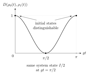
For inputs $|0\rangle$ and $|1\rangle$, the trace distance $D(\rho_0,\rho_1)=\tfrac12\|\rho_0-\rho_1\|_1$ equals $\cos^2(gt)$. Both reduced states become $I/2$, then separate again. The joint evolution retains the information needed for this revival.

Thus each $\Phi_t$ is CPTP, but this family is neither a semigroup nor CP divisible throughout the evolution. It also has no regular time-local generator at the instant when it erases all system information. On invertible intervals a time-local generator may exist without representing memoryless physics; see Time-Convolutionless Master Equations.

A time-homogeneous quantum dynamical semigroup has the stronger property $\Phi_{t+s}=\Phi_t\Phi_s$ and, in finite dimension with continuity, $\Phi_t=e^{t\mathcal L}$ with a GKSL generator. Memory-kernel and multi-time descriptions handle more general behavior. The Schwinger–Keldysh bridge describes the related influence-functional approach for fields.

Exercises

1. Kraus operators from a unitary dilation. Starting from

$$\Phi(\rho) = \operatorname{Tr}_E \left[ U(\rho\otimes\eta_E)U^\dagger \right],$$

with $\eta_E=\sum_rq_r|r\rangle\langle r|$, derive the Kraus operators $K_{\mu r}=\sqrt{q_r}\langle\mu|U|r\rangle$.

Solution

Insert the spectral decomposition of $\eta_E$:

$$\Phi(\rho) = \sum_r q_r \operatorname{Tr}_E \left[ U(\rho\otimes|r\rangle\langle r|)U^\dagger \right].$$

Now evaluate the partial trace in the basis $\{|\mu\rangle\}$:

$$\Phi(\rho) = \sum_{\mu,r}q_r \langle\mu|U|r\rangle \rho \langle r|U^\dagger|\mu\rangle.$$

Defining

$$K_{\mu r} = \sqrt{q_r}\langle\mu|U|r\rangle$$

gives

$$\Phi(\rho) = \sum_{\mu,r}K_{\mu r}\rho K_{\mu r}^\dagger.$$

2. Trace preservation. Prove that the Kraus operators in the previous exercise satisfy $\sum_{\mu,r}K_{\mu r}^\dagger K_{\mu r}=I_S$.

Solution

Using the definition,

$$\sum_{\mu,r}K_{\mu r}^\dagger K_{\mu r} = \sum_{\mu,r} q_r \langle r|U^\dagger|\mu\rangle \langle\mu|U|r\rangle.$$

The sum over $\mu$ gives the identity on the environment:

$$\sum_\mu|\mu\rangle\langle\mu|=I_E.$$

Thus

$$\sum_{\mu,r}K_{\mu r}^\dagger K_{\mu r} = \sum_r q_r \langle r|U^\dagger U|r\rangle = \sum_r q_r I_S =I_S.$$

3. Initial correlations can matter. Let $S$ and $E$ be qubits. Define two initial total states

$$\rho_{SE}^{(A)} = \frac12|00\rangle\langle00| + \frac12|11\rangle\langle11|,$$

and

$$\rho_{SE}^{(B)} = \frac12|01\rangle\langle01| + \frac12|10\rangle\langle10|.$$

Both have $\rho_S=I/2$. Let $U$ flip $S$ if $E=1$ and do nothing if $E=0$. Compute the final reduced state of $S$ for each initial total state.

Solution

The unitary acts as

$$|s,e\rangle \longmapsto |s\oplus e,e\rangle.$$

For $\rho_{SE}^{(A)}$, the components transform as

$$|00\rangle\to|00\rangle, \qquad |11\rangle\to|01\rangle.$$

Both final components have $S=0$, so

$$\rho_S^{(A)}(t) = |0\rangle\langle0|.$$

For $\rho_{SE}^{(B)}$,

$$|01\rangle\to|11\rangle, \qquad |10\rangle\to|10\rangle.$$

Both final components have $S=1$, so

$$\rho_S^{(B)}(t) = |1\rangle\langle1|.$$

The same initial reduced state $\rho_S=I/2$ led to different final reduced states because the hidden initial correlations were different. Therefore no map of $\rho_S$ alone can describe both cases.

References

• H.-P. Breuer and F. Petruccione, The Theory of Open Quantum Systems, Oxford University Press (2002). Publisher.
• I. de Vega and D. Alonso, “Dynamics of non-Markovian open quantum systems,” Reviews of Modern Physics 89, 015001 (2017). Author manuscript.
• K. Kraus, States, Effects, and Operations: Fundamental Notions of Quantum Theory, Springer (1983). Publisher.
• Á. Rivas and S. F. Huelga, Open Quantum Systems: An Introduction, Springer (2012). Author manuscript.
• H. M. Wiseman and G. J. Milburn, Quantum Measurement and Control, Cambridge University Press (2010). Publisher.