Momentum-Space Many-Body Hamiltonians

Momentum space turns spatial translation structure into algebra on mode labels. A translation-invariant one-body kernel becomes diagonal in wave vector, while a translation-invariant interaction becomes a vertex that preserves the sum of incoming and outgoing momenta. On a lattice, the corresponding label is crystal momentum, defined only modulo a reciprocal-lattice vector.

The basic tradeoff is

$$\text{locality in real space} \quad\longleftrightarrow\quad \text{broad coupling in momentum space},$$

whereas convolution or translation invariance in real space becomes multiplication or a conservation delta in momentum space.

This page develops many-body Hamiltonians and Fock-space operators in momentum representation. One-particle amplitudes and their Born interpretation live in Momentum-Space Representation. Transform calculations live in Position and Momentum Representations, and the transform signs are explained in Fourier Transform Conventions. The complementary continuum-cell-lattice dictionary is developed in Real-Space Representation.

Helpful background. Fourier conventions fixes the transform pair; field applications explains the mode expansion; two-body operators explains pair coefficients.

Plane-wave modes in a periodic box

Use a $d$-dimensional box of volume $\mathcal V=L^d$. The label $\mathbf k$ is a wave vector; the translation momentum is $\hbar\mathbf k$, equal to mechanical momentum for the free continuum particles considered here, without a gauge potential. Internal labels $\alpha,\beta$ include any spin or orbital index and are summed only when shown. Write $[A,B]_{\mp}=AB\mp BA$, with the upper sign for bosons and lower sign for fermions.

Periodic boundary conditions make plane waves orthogonal and translation symmetry exact. Traps, disorder and open boundaries can still be represented in a Fourier basis, but the transformed Hamiltonian generally mixes its labels.

Transform and inverse

In a cubic periodic box of volume $\mathcal V=L^d$,

$$\psi_\alpha(\mathbf r) = \frac1{\sqrt{\mathcal V}} \sum_{\mathbf k} e^{i\mathbf k\cdot\mathbf r} a_{\mathbf k\alpha}.$$

The inverse transform is

$$a_{\mathbf k\alpha} = \frac1{\sqrt{\mathcal V}} \int_{\mathcal V} d^dr\, e^{-i\mathbf k\cdot\mathbf r} \psi_\alpha(\mathbf r).$$

Periodic boundary conditions quantize the wave vectors:

$$\mathbf k = \frac{2\pi}{L} \mathbf n, \qquad \mathbf n\in\mathbb Z^d.$$

For a rectangular box, replace $2\pi n_\mu/L$ by $2\pi n_\mu/L_\mu$ in each direction.

Orthogonality and completeness

The plane-wave modes satisfy

$$\int_{\mathcal V} d^dr\, e^{i(\mathbf k-\mathbf k')\cdot\mathbf r} = \mathcal V \delta_{\mathbf k,\mathbf k'}.$$

The periodic delta distribution is

$$\delta_{\mathcal V}(\mathbf r-\mathbf r') = \frac1{\mathcal V} \sum_{\mathbf k} e^{i\mathbf k\cdot(\mathbf r-\mathbf r')}.$$

It acts as the identity on functions compatible with the periodic box.

Canonical algebra

If the equal-time field algebra is

$$[\psi_\alpha(\mathbf r), \psi_\beta^\dagger(\mathbf r')]_{\mp} = \delta_{\alpha\beta} \delta_{\mathcal V}(\mathbf r-\mathbf r'),$$

then the mode operators obey

$$[a_{\mathbf k\alpha}, a_{\mathbf k'\beta}^\dagger]_{\mp} = \delta_{\mathbf k,\mathbf k'} \delta_{\alpha\beta}.$$

All same-type mode brackets vanish. The Fourier transform is unitary on the retained one-particle space, so it preserves bosonic or fermionic statistics.

Continuum Transform

In infinite volume write $\int_{\mathbf k}\equiv\int d^dk/(2\pi)^d$ and use

$$\psi_\alpha(\mathbf r) = \int_{\mathbf k} e^{i\mathbf k\cdot\mathbf r} a_\alpha(\mathbf k),$$

with inverse

$$a_\alpha(\mathbf k) = \int d^dr\, e^{-i\mathbf k\cdot\mathbf r} \psi_\alpha(\mathbf r).$$

The continuum mode algebra is

$$[a_\alpha(\mathbf k), a_\beta^\dagger(\mathbf k')]_{\mp} = (2\pi)^d \delta_{\alpha\beta} \delta^{(d)}(\mathbf k-\mathbf k').$$

The mode operator $a_\alpha(\mathbf k)$ is distribution valued. It is not the same dimensionless object as the finite-box $a_{\mathbf k\alpha}$.

Box-to-Continuum Dictionary

The thermodynamic-limit replacements are

$$\frac1{\mathcal V} \sum_{\mathbf k} \longrightarrow \int_{\mathbf k},$$

and, schematically at the allowed box momenta,

$$a_\alpha(\mathbf k) \longleftrightarrow \sqrt{\mathcal V} a_{\mathbf k\alpha}.$$

Correspondingly,

$$(2\pi)^d \delta^{(d)}(\mathbf k-\mathbf k') \longleftrightarrow \mathcal V \delta_{\mathbf k,\mathbf k'}.$$

These replacements must be applied consistently to the integration measure, delta functions, operators, and interaction prefactors. Mixing one box convention with one continuum convention is a common source of missing powers of volume.

Particle Number in Momentum Space

The total number operator is basis invariant:

$$\widehat N = \sum_{\mathbf k,\alpha} a_{\mathbf k\alpha}^\dagger a_{\mathbf k\alpha}$$

in a finite box, or

$$\widehat N = \sum_\alpha \int_{\mathbf k} a_\alpha^\dagger(\mathbf k) a_\alpha(\mathbf k)$$

in the continuum convention above.

Individual occupations

$$n_{\mathbf k\alpha} = a_{\mathbf k\alpha}^\dagger a_{\mathbf k\alpha}$$

need not be conserved when interactions scatter particles between momenta.

Kinetic Energy Becomes Diagonal

For nonrelativistic particles,

$$T = \sum_\alpha \int d^dr\, \psi_\alpha^\dagger(\mathbf r) \left( -\frac{\hbar^2\nabla^2}{2m_\alpha} \right) \psi_\alpha(\mathbf r).$$

Since

$$-\nabla^2 e^{i\mathbf k\cdot\mathbf r} = k^2 e^{i\mathbf k\cdot\mathbf r},$$

orthogonality gives

$$T = \sum_{\mathbf k,\alpha} \varepsilon_\alpha(\mathbf k) a_{\mathbf k\alpha}^\dagger a_{\mathbf k\alpha},$$

where

$$\varepsilon_\alpha(\mathbf k) = \frac{\hbar^2k^2}{2m_\alpha}.$$

The diagonalization follows from translation invariance and the plane-wave eigenvalue of $-\nabla^2$.

General Translation-Invariant One-Body Kernel

Consider

$$H_1 ={} \sum_{\alpha,\beta} \int d^dr\,d^dr'\, \psi_\alpha^\dagger(\mathbf r) \times h_{\alpha\beta}(\mathbf r-\mathbf r') \psi_\beta(\mathbf r').$$

The dependence only on $\mathbf r-\mathbf r'$ expresses continuous translation invariance. Hermiticity requires $h_{\alpha\beta}(\mathbf x)=h_{\beta\alpha}(-\mathbf x)^*$. In a finite periodic box use the corresponding periodic kernel and integrate over the box; in infinite space replace the momentum sum below by $\int_{\mathbf k}$. Fourier transformation gives

$$H_1 = \sum_{\mathbf k} \sum_{\alpha,\beta} a_{\mathbf k\alpha}^\dagger h_{\alpha\beta}(\mathbf k) a_{\mathbf k\beta},$$

where

$$h_{\alpha\beta}(\mathbf k) = \int d^dx\, e^{-i\mathbf k\cdot\mathbf x} h_{\alpha\beta}(\mathbf x).$$

Momentum is diagonal, but internal labels can still mix through the matrix $h(\mathbf k)$.

Bands and Internal Components

At each $\mathbf k$, diagonalize the Hermitian matrix

$$h(\mathbf k) u_n(\mathbf k) = \varepsilon_n(\mathbf k) u_n(\mathbf k).$$

Defining band operators

$$\gamma_{n\mathbf k} = \sum_\alpha u_{n\alpha}(\mathbf k)^* a_{\mathbf k\alpha}$$

gives

$$H_1 = \sum_{n,\mathbf k} \varepsilon_n(\mathbf k) \gamma_{n\mathbf k}^\dagger \gamma_{n\mathbf k}.$$

Fourier transformation and band diagonalization are separate steps. A lattice Fourier transform resolves translation sectors; a $\mathbf k$-dependent unitary resolves orbital or sublattice mixing inside each sector.

Total Momentum Operator

For a translation-invariant continuum model,

$$\mathbf P = \sum_{\mathbf k,\alpha} \hbar\mathbf k\, a_{\mathbf k\alpha}^\dagger a_{\mathbf k\alpha}.$$

It acts on ladder operators as

$$[\mathbf P,a_{\mathbf k\alpha}^\dagger] = \hbar\mathbf k\, a_{\mathbf k\alpha}^\dagger,$$

and

$$[\mathbf P,a_{\mathbf k\alpha}] = -\hbar\mathbf k\, a_{\mathbf k\alpha}.$$

Thus a Fock basis vector has total momentum

$$\mathbf P_{\boldsymbol n} = \sum_{\mathbf k,\alpha} \hbar\mathbf k\, n_{\mathbf k\alpha}.$$

Momentum Charge of an Operator String

For

$$M = a_{\mathbf k_1}^\dagger \cdots a_{\mathbf k_p}^\dagger a_{\mathbf q_s} \cdots a_{\mathbf q_1},$$

the commutator is

$$\begin{aligned} [\mathbf P,M] ={}& \hbar \left( \sum_{i=1}^{p}\mathbf k_i - \sum_{j=1}^{s}\mathbf q_j \right) M. \end{aligned}$$

A nonzero string preserves total momentum exactly when the created and annihilated wave-vector sums agree.

This is the momentum analogue of number-charge counting in Number Operators and Conserved Quantities.

Translation Symmetry and Momentum Blocks

If

$$[H,\mathbf P] = 0,$$

then the Hamiltonian is block diagonal in total-momentum sectors. A state initialized in one sector remains there under closed-system evolution.

The converse practical warning is important: writing operators with momentum labels does not guarantee momentum conservation. External traps, boundaries, disorder, drives, or inconsistent cutoffs can connect different total momenta.

The symmetry derivation is given in Translation-Invariant Hamiltonians.

Translationally Invariant Pair Interaction

Let

$$H_{\mathrm{int}} ={} \frac12 \sum_{\alpha,\beta} \int d^dr\,d^dr'\, \psi_\alpha^\dagger(\mathbf r) \psi_\beta^\dagger(\mathbf r') \times v_{\alpha\beta}(\mathbf r-\mathbf r') \psi_\beta(\mathbf r') \psi_\alpha(\mathbf r).$$

Define

$$\widetilde v_{\alpha\beta}(\mathbf q) = \int d^dx\, e^{-i\mathbf q\cdot\mathbf x} v_{\alpha\beta}(\mathbf x).$$

For the box, take the periodic continuation of the pair potential. Its Fourier coefficient is the integral over one cell; for a convergent periodization it equals the displayed infinite-space transform at the allowed wave vectors. Assume $v_{\alpha\beta}(\mathbf x)$ is real and $v_{\alpha\beta}(\mathbf x)=v_{\beta\alpha}(-\mathbf x)$, so the pair interaction is Hermitian and exchange symmetric. The finite-box form is

$$H_{\mathrm{int}} ={} \frac1{2\mathcal V} \sum_{\substack{\mathbf k_1,\mathbf k_2,\\ \mathbf k_3,\mathbf k_4}} \sum_{\alpha,\beta} \delta_{\mathbf k_1+\mathbf k_2, \mathbf k_3+\mathbf k_4} \times \widetilde v_{\alpha\beta} (\mathbf k_1-\mathbf k_3) a_{\mathbf k_1\alpha}^\dagger a_{\mathbf k_2\beta}^\dagger a_{\mathbf k_4\beta} a_{\mathbf k_3\alpha}.$$

Under this Fourier convention, $\widetilde v(\mathbf q)$ has units of energy times volume. The combination $\widetilde v(\mathbf q)/\mathcal V$ multiplying the dimensionless mode operators therefore has units of energy, as the Hamiltonian requires.

The Kronecker delta comes from integrating a common spatial translation of both particles. It enforces equality of total incoming and outgoing momentum.

Momentum-Transfer Form

Set

$$\mathbf k_3=\mathbf k, \qquad \mathbf k_4=\mathbf k',$$

and define the wave-vector transfer

$$\mathbf q = \mathbf k_1-\mathbf k.$$

The momentum transferred is $\hbar\mathbf q$. Momentum conservation fixes the other outgoing wave vector to $\mathbf k'-\mathbf q$. Therefore

$$H_{\mathrm{int}} ={} \frac1{2\mathcal V} \sum_{\mathbf k,\mathbf k',\mathbf q} \sum_{\alpha,\beta} \widetilde v_{\alpha\beta}(\mathbf q) \times a_{\mathbf k+\mathbf q,\alpha}^\dagger a_{\mathbf k'-\mathbf q,\beta}^\dagger a_{\mathbf k'\beta} a_{\mathbf k\alpha}.$$

Every term visibly satisfies

$$(\mathbf k+\mathbf q) + (\mathbf k'-\mathbf q) = \mathbf k+\mathbf k'.$$

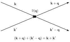
A translation-invariant two-body vertex transfers momentum $\hbar\mathbf q$ from one line to the other. Individual momenta change, but the sum of the two outgoing wave vectors equals the sum of the two incoming wave vectors.

Ordered and Antisymmetrized Vertices

The displayed pair interaction uses ordered two-particle matrix elements and the prefactor $1/2$. For identical fermions one may instead use an antisymmetrized vertex,

$$\overline{\mathcal V}_{12;34} = \mathcal V_{12;34} - \mathcal V_{12;43},$$

with the prefactor $1/4$. Direct and exchange transfer channels are then packaged into $\overline{\mathcal V}$.

These prefactors must follow the coefficient convention, not visual inspection of the quartic string. The coefficient comparison is in Two-Body Operators.

Contact Interaction

For

$$v(\mathbf r) = g\delta^{(d)}(\mathbf r),$$

the Fourier transform is independent of transfer:

$$\widetilde v(\mathbf q) = g.$$

Hence

$$H_{\mathrm{contact}} ={} \frac{g}{2\mathcal V} \sum_{\mathbf k,\mathbf k',\mathbf q} a_{\mathbf k+\mathbf q}^\dagger a_{\mathbf k'-\mathbf q}^\dagger \times a_{\mathbf k'} a_{\mathbf k}.$$

A constant momentum-space vertex does not mean that the particles do not scatter. It means that the idealized zero-range interaction has no transfer dependence before regularization.

This single-component contact term is useful for bosons. For a single complete fermion component the local quartic product vanishes by antisymmetry; ordinary fermionic s-wave contact scattering needs different internal components. Where a continuum contact interaction is ultraviolet sensitive, the bare coupling depends on the regulator and must be matched to scattering data.

Density Modes

Define the Fourier component of number density by

$$\rho_{\mathbf q} = \sum_{\mathbf k,\alpha} a_{\mathbf k+\mathbf q,\alpha}^\dagger a_{\mathbf k\alpha}.$$

With

$$n(\mathbf r) = \sum_\alpha \psi_\alpha^\dagger(\mathbf r) \psi_\alpha(\mathbf r),$$

the box Fourier pair is

$$\begin{aligned} n(\mathbf r) &= \frac1{\mathcal V} \sum_{\mathbf q} e^{-i\mathbf q\cdot\mathbf r} \rho_{\mathbf q}, \\ \rho_{\mathbf q} &= \int_{\mathcal V}d^dr\, e^{i\mathbf q\cdot\mathbf r} n(\mathbf r). \end{aligned}$$

It satisfies

$$\rho_{\mathbf q}^\dagger = \rho_{-\mathbf q},$$

and

$$\rho_{\mathbf0} = \widehat N.$$

The momentum carried by the density mode is

$$[\mathbf P,\rho_{\mathbf q}] = \hbar\mathbf q\, \rho_{\mathbf q}.$$

Thus $\rho_{\mathbf q}$ transfers wave vector $\mathbf q$ without changing particle number. Its Fourier integral has a plus sign because we chose the momentum-raising bilinear. Authors defining the density transform with a minus sign call this same operator $\rho_{-\mathbf q}$; translate the label before comparing response functions.

Interaction in Density Form

For a spin-independent pair potential,

$$H_{\mathrm{int}} = \frac1{2\mathcal V} \sum_{\mathbf q} \widetilde v(\mathbf q) :\rho_{\mathbf q} \rho_{-\mathbf q}:_0.$$

The empty-vacuum normal ordering removes the one-particle self-contraction and reproduces the pair interaction. With the complete momentum sums used here, $\rho_{\mathbf q}\rho_{-\mathbf q}=:\rho_{\mathbf q}\rho_{-\mathbf q}:_0+\widehat N$. The subtraction removes the same particle appearing twice. After a momentum cutoff the contraction is restricted by the retained modes and is not automatically the full $\widehat N$ for every $\mathbf q$. Long-range Coulomb models also need a specified neutralizing background and treatment of the zero-transfer term; normal ordering alone does not supply them.

Density modes are the natural operators for structure factors and density response, developed from the correlation side in Density Operators and Current Operators.

Momentum Distribution

For a state $\rho$, define

$$n_\alpha(\mathbf k) = \langle a_{\mathbf k\alpha}^\dagger a_{\mathbf k\alpha} \rangle.$$

Then

$$\langle\widehat N\rangle = \sum_{\mathbf k,\alpha} n_\alpha(\mathbf k).$$

For a translation-invariant state, the one-body momentum density matrix is diagonal between distinct translation characters:

$$\langle a_{\mathbf k\alpha}^\dagger a_{\mathbf k'\beta} \rangle \propto \delta_{\mathbf k,\mathbf k'}.$$

Internal labels can remain off diagonal. Translation breaking at wave vector $\mathbf Q$ can instead produce coherence between $\mathbf k$ and $\mathbf k+\mathbf Q$.

External Potentials Mix Momenta

For a one-body external potential,

$$H_U = \sum_\alpha \int d^dr\, U(\mathbf r) \psi_\alpha^\dagger(\mathbf r) \psi_\alpha(\mathbf r),$$

define

$$\widetilde U(\mathbf q) = \int d^dr\, e^{-i\mathbf q\cdot\mathbf r} U(\mathbf r).$$

In a box,

$$H_U = \frac1{\mathcal V} \sum_{\mathbf k,\mathbf k',\alpha} \widetilde U(\mathbf k-\mathbf k') a_{\mathbf k\alpha}^\dagger a_{\mathbf k'\alpha}.$$

A constant potential contributes only at zero transfer and remains diagonal. A trap or impurity contains many Fourier components and mixes momenta. A periodic potential couples momenta separated by reciprocal-lattice vectors.

Center-of-Mass and Relative Momentum

For two particles, define

$$\mathbf K = \mathbf k_1+\mathbf k_2$$

and, for equal masses,

$$\mathbf k_{\mathrm{rel}} = \frac12 (\mathbf k_1-\mathbf k_2).$$

A translation-invariant pair interaction preserves $\mathbf K$ while changing relative momentum. The transfer variable $\mathbf q$ acts within a fixed center-of-mass sector.

For unequal masses, the mass-weighted relative coordinate and momentum should be used. The equal-mass half-difference is not universal.

Finite Volume and the Thermodynamic Limit

Periodic finite volume replaces integrals by discrete sums and Dirac deltas by Kronecker deltas. This is useful computationally and regulates infrared questions. The limit

$$L\to\infty$$

at fixed density makes the momentum grid dense:

$$\Delta k = \frac{2\pi}{L} \longrightarrow 0.$$

The ultraviolet range is a separate issue. Increasing $L$ at fixed spatial mesh spacing improves infrared resolution but does not automatically raise the momentum cutoff.

Lattice Fourier Transform

For a periodic Bravais lattice with $N_s$ cells at positions $\mathbf R_j$, define

$$a_{\mathbf k\alpha} = \frac1{\sqrt{N_s}} \sum_j e^{-i\mathbf k\cdot\mathbf R_j} a_{j\alpha},$$

and

$$a_{j\alpha} = \frac1{\sqrt{N_s}} \sum_{\mathbf k\in\mathrm{BZ}} e^{i\mathbf k\cdot\mathbf R_j} a_{\mathbf k\alpha}.$$

The allowed $\mathbf k$ values are the discrete translation characters compatible with the finite periodic lattice. The transform preserves the canonical mode algebra.

Translation-Invariant Hopping

Let

$$H_t = - \sum_{j,\boldsymbol\delta,\alpha} t_\alpha(\boldsymbol\delta) a_{j+\boldsymbol\delta,\alpha}^\dagger a_{j\alpha}.$$

Translation invariance means the hopping depends on displacement $\boldsymbol\delta$, not on $j$. Fourier transformation gives

$$H_t = \sum_{\mathbf k,\alpha} \varepsilon_\alpha(\mathbf k) a_{\mathbf k\alpha}^\dagger a_{\mathbf k\alpha},$$

with

$$\varepsilon_\alpha(\mathbf k) = - \sum_{\boldsymbol\delta} t_\alpha(\boldsymbol\delta) e^{-i\mathbf k\cdot\boldsymbol\delta}.$$

Hermiticity requires

$$t_\alpha(-\boldsymbol\delta) = t_\alpha(\boldsymbol\delta)^*,$$

which makes $\varepsilon_\alpha(\mathbf k)$ real.

Nearest-Neighbor Chain

For a one-dimensional chain with spacing $a$ and real nearest-neighbor hopping $t$,

$$H_t = -t \sum_j \left( a_{j+1}^\dagger a_j + a_j^\dagger a_{j+1} \right).$$

The dispersion is

$$\varepsilon(k) = -2t\cos(ka).$$

Momentum space diagonalizes the quadratic hopping, but the cosine remembers the finite lattice spacing and bounded Brillouin zone. The model-level derivation, open and twisted chains, bandwidth, effective mass, and multi-orbital extension live in Tight-Binding Model.

Multi-Orbital Unit Cells

With several orbitals or sublattices per cell,

$$H_0 = \sum_{\mathbf k} \sum_{\alpha,\beta} a_{\mathbf k\alpha}^\dagger h_{\alpha\beta}(\mathbf k) a_{\mathbf k\beta}.$$

The matrix $h(\mathbf k)$ is not generally diagonal. Its eigenvalues are bands, while its eigenvectors carry orbital composition.

Two common Fourier conventions use phases based on either the cell position $\mathbf R_j$ or the full orbital position $\mathbf R_j+\mathbf r_\alpha$. They differ by a $\mathbf k$-dependent diagonal unitary. Matrix entries and eigenvector phases change, while physical spectra and consistently computed observables do not.

Transforming an interaction from orbital operators to band operators inserts products of these eigenvectors as form factors. Consequently, even an onsite interaction that is momentum independent in the orbital basis generally acquires momentum and band dependence in the band basis.

Brillouin-Zone Preview

Reciprocal-lattice vectors satisfy

$$e^{i\mathbf G\cdot\mathbf R_j} = 1$$

for every Bravais-lattice vector $\mathbf R_j$. Therefore

$$\mathbf k \sim \mathbf k+\mathbf G.$$

A Brillouin zone chooses one representative from each equivalence class. In a one-dimensional lattice of spacing $a$, a standard first zone is

$$-\frac{\pi}{a} \le k < \frac{\pi}{a}.$$

The endpoints are equivalent. The Brillouin zone is not a hard wall in physical momentum; it is a fundamental domain for the crystal-momentum label.

Brillouin-Zone Integration

If the unit-cell volume is $v_c$, then

$$\operatorname{Vol}(\mathrm{BZ}) = \frac{(2\pi)^d}{v_c}.$$

In the large-lattice limit,

$$\frac1{N_s} \sum_{\mathbf k\in\mathrm{BZ}} \longrightarrow \frac{v_c}{(2\pi)^d} \int_{\mathrm{BZ}} d^dk.$$

This normalization is distinct from the continuum free-space integral when internal bands and unit-cell volumes are present.

Crystal-Momentum Conservation

Discrete translation symmetry conserves total crystal momentum only modulo a reciprocal vector:

$$\mathbf k_1+\mathbf k_2 - \mathbf k_3-\mathbf k_4 = \mathbf G.$$

Equivalently, the phase under every lattice translation is conserved. Folding all labels into one Brillouin zone can make a nonzero $\mathbf G$ appear in the representative equation even though the translation character is unchanged.

Crystal momentum should not be identified automatically with the total mechanical momentum of particles plus lattice.

Onsite Hubbard Interaction

For spin-$1/2$ fermions,

$$H_U = U \sum_j n_{j\uparrow}n_{j\downarrow}.$$

Its momentum-space form is

$$H_U ={} \frac{U}{N_s} \sum_{\mathbf k,\mathbf k',\mathbf q} c_{\mathbf k+\mathbf q,\uparrow}^\dagger c_{\mathbf k'-\mathbf q,\downarrow}^\dagger \times c_{\mathbf k',\downarrow} c_{\mathbf k,\uparrow},$$

where all labels are understood modulo reciprocal vectors or accompanied by the appropriate crystal-momentum delta.

An onsite interaction is local in the site basis but couples every allowed transfer $\mathbf q$ in the momentum basis.

Bose–Hubbard Interaction

The Bose–Hubbard model uses the following onsite vertex in addition to hopping.

For onsite bosons,

$$H_U^{(B)} = \frac U2 \sum_j n_j(n_j-1),$$

and

$$H_U^{(B)} ={} \frac{U}{2N_s} \sum_{\mathbf k,\mathbf k',\mathbf q} b_{\mathbf k+\mathbf q}^\dagger b_{\mathbf k'-\mathbf q}^\dagger \times b_{\mathbf k'} b_{\mathbf k}.$$

The factor $1/2$ avoids double counting identical boson pairs. The momentum-independent onsite vertex still generates nontrivial scattering and correlations.

Normal and Umklapp Processes

When all crystal momenta are represented in the first Brillouin zone:

• a normal process has $\mathbf G=\mathbf0$;
• an Umklapp process has $\mathbf G\neq\mathbf0$.

Umklapp is allowed by lattice translation symmetry because reciprocal vectors have trivial translation phase. Its effect on current or transport depends on the full model, occupations, dimensionality, and available phase space. The word does not by itself prove a finite resistivity.

Twisted Boundary Conditions

For a spatial twist $\boldsymbol\theta$,

$$\psi(\mathbf r+L\mathbf e_\mu) = e^{i\theta_\mu} \psi(\mathbf r).$$

The allowed components become

$$k_\mu = \frac{2\pi n_\mu+\theta_\mu}{L}.$$

Twists shift the finite-size momentum grid and are useful for flux insertion, stiffness, and boundary-condition averaging. A spatial antiperiodic boundary condition corresponds to $\theta_\mu=\pi$.

Do not confuse spatial twists with the bosonic or fermionic boundary conditions imposed in imaginary time at finite temperature.

Open Boundaries

With open boundaries, ordinary plane waves need not diagonalize the one-body Hamiltonian. Standing waves, sine transforms, or direct real-space methods may be natural. One may still Fourier transform data, but the resulting momentum labels are not exact translation quantum numbers.

Boundary terms also matter when deriving momentum conservation. A finite open sample can exchange momentum with its boundaries.

Momentum cutoffs and aliasing

Retaining plane waves from a set $S$, such as $|\mathbf k|\le\Lambda$, projects onto a translation-invariant one-particle subspace. Any such projector commutes with translations, even if $S$ is asymmetric. An asymmetric set can break inversion or rotational symmetry; it does not by itself break translation symmetry. A consistently projected interaction still preserves the exact continuum momentum of every retained matrix element.

Products generate wave vectors outside $S$. A Galerkin projection discards those components. Evaluating the product on a finite spatial grid can instead alias them into retained modes, identifying wave vectors modulo the sampling reciprocal vector. That wraparound is appropriate for an actual lattice model but can create spurious momentum transfers in a continuum calculation. De-aliasing or a sufficiently enlarged product grid avoids this confusion.

The cutoff also changes virtual scattering and may require coupling matching. Integrating out discarded modes can generate effective higher-body interactions; simply deleting their basis states is a different approximation. Infrared resolution, ultraviolet matching and aliasing are separate checks.

Continuum and Lattice Comparison

Feature	Continuum	Periodic lattice
translation group	continuous	discrete Bravais lattice
label	translation wave vector, with momentum $\hbar\mathbf k$	crystal momentum
equivalence	unique in reciprocal space	$\mathbf k\sim\mathbf k+\mathbf G$
domain	all $\mathbb R^d$ before cutoff	one Brillouin zone
kinetic term	often $\hbar^2k^2/(2m)$	band dispersion $\varepsilon_n(\mathbf k)$
conserved sum	exact momentum	crystal momentum modulo $\mathbf G$
local interaction prefactor	typically $1/\mathcal V$	typically $1/N_s$

The two descriptions approach one another only in a stated continuum limit near selected low-energy momenta.

Exercises

Interaction conservation delta

Show that the coordinate integral in a translation-invariant pair interaction produces

$$\mathcal V\delta_{\mathbf k_1+\mathbf k_2, \mathbf k_3+\mathbf k_4} \widetilde v(\mathbf k_1-\mathbf k_3).$$

Solution

The relevant integral is

$$I ={} \int d^dr\,d^dr'\, e^{-i\mathbf k_1\cdot\mathbf r} e^{-i\mathbf k_2\cdot\mathbf r'} \times v(\mathbf r-\mathbf r') e^{i\mathbf k_4\cdot\mathbf r'} e^{i\mathbf k_3\cdot\mathbf r}.$$

Set $\mathbf x=\mathbf r-\mathbf r'$ and keep $\mathbf r'$ as the center coordinate. The exponent becomes

$$-i(\mathbf k_1-\mathbf k_3)\cdot\mathbf x - i(\mathbf k_1+\mathbf k_2 -\mathbf k_3-\mathbf k_4) \cdot\mathbf r'.$$

The $\mathbf x$ integral gives $\widetilde v(\mathbf k_1-\mathbf k_3)$. The center-coordinate integral gives

$$\mathcal V \delta_{\mathbf k_1+\mathbf k_2, \mathbf k_3+\mathbf k_4}.$$

Combining this factor with the four field normalizations leaves the overall $1/\mathcal V$ vertex prefactor.

Hubbard vertex

Transform $U\sum_jn_{j\uparrow}n_{j\downarrow}$ to momentum space and identify the conserved crystal-momentum combination.

Solution

Insert four lattice transforms. The site sum produces

$$\sum_j e^{i(-\mathbf k_1-\mathbf k_2 +\mathbf k_3+\mathbf k_4)\cdot\mathbf R_j} = N_s \delta^{(\mathbf G)}_{\mathbf k_1+\mathbf k_2, \mathbf k_3+\mathbf k_4}.$$

Three independent sums remain. Writing the transfer as $\mathbf q$ gives

$$H_U ={} \frac U{N_s} \sum_{\mathbf k,\mathbf k',\mathbf q} c_{\mathbf k+\mathbf q,\uparrow}^\dagger c_{\mathbf k'-\mathbf q,\downarrow}^\dagger \times c_{\mathbf k',\downarrow} c_{\mathbf k,\uparrow}.$$

The conserved combination is

$$\mathbf k_1+\mathbf k_2 - \mathbf k_3-\mathbf k_4 = \mathbf G.$$

Twisted momentum grid

For

$$\psi(x+L) = e^{i\theta} \psi(x),$$

derive the allowed $k$ values and recover periodic and antiperiodic cases.

Solution

A plane wave satisfies

$$e^{ik(x+L)} = e^{ikL}e^{ikx}.$$

The boundary condition requires

$$e^{ikL} = e^{i\theta}.$$

Therefore

$$kL = 2\pi n+\theta,$$

or

$$k_n = \frac{2\pi n+\theta}{L}.$$

Periodic boundaries have $\theta=0$. Spatial antiperiodic boundaries have $\theta=\pi$, shifting the grid by half a spacing.

A continuum product and its aliased image

On a periodic interval of length $2\pi$, retain wave numbers $-2,-1,0,1,2$. The function $f(x)=e^{2ix}$ lies in this space. Compare the projected product $P[f^2]$ with its representation from five equally spaced sample points.

Solution

The exact square is $e^{4ix}$, so its orthogonal projection onto the retained modes is zero. At $x_j=2\pi j/5$, however, $e^{4ix_j}=e^{-ix_j}$. A five-point discrete transform therefore reports the retained mode $k=-1$. It has replaced wave-number addition by addition modulo five. That describes the translation characters of a five-site lattice, but is not the continuum Galerkin product.

References

• A. Altland and B. Simons, Condensed Matter Field Theory, 2nd ed., Cambridge University Press (2010).
• N. W. Ashcroft and N. D. Mermin, Solid State Physics, Holt, Rinehart and Winston (1976).
• H. Bruus and K. Flensberg, Many-Body Quantum Theory in Condensed Matter Physics, Oxford University Press (2004).
• P. Coleman, Introduction to Many-Body Physics, Cambridge University Press (2015).
• A. L. Fetter and J. D. Walecka, Quantum Theory of Many-Particle Systems, Dover (2003).
• E. Fradkin, Field Theories of Condensed Matter Physics, 2nd ed., Cambridge University Press (2013), doi:10.1017/CBO9781139015509.
• T. Giamarchi, Quantum Physics in One Dimension, Oxford University Press (2004).
• G. D. Mahan, Many-Particle Physics, 3rd ed., Springer (2000).
• J. W. Negele and H. Orland, Quantum Many-Particle Systems, Westview Press (1998).
• L. Pitaevskii and S. Stringari, Bose–Einstein Condensation and Superfluidity, Oxford University Press (2016).