From Matter Waves to Schrödinger Equation

Matter waves made a new mechanics plausible. If material particles carry phase and wavelength, then a theory of particles should look partly like a wave theory. Schrödinger’s equation was the decisive step: it turned the de Broglie relations into a differential equation that could calculate spectra, scattering, wave packets, and tunneling.

The plane-wave argument below motivates the equation but does not derive all of quantum theory. To solve initial-value problems, continue with Time-Dependent Schrödinger Equation and Schrödinger Equation. The historical page is Schrödinger’s Wave Mechanics.

Momentum-Wavelength Relation

The de Broglie relation assigns a wavelength to a particle of momentum $p$:

$$\lambda = \frac{h}{p}.$$

Equivalently, using $k=2\pi/\lambda$,

$$p = \hbar k.$$

This relation made electron diffraction intelligible. A beam of electrons accelerated through a voltage has a calculable momentum, and hence a calculable wavelength. Crystal scattering then tests whether that wavelength appears in diffraction. See de Broglie Matter Waves and Electron Diffraction.

The modern interpretation is sharper: plane waves are momentum eigenstate idealizations, and localized particles require wave packets. The wavelength is not a literal water-wave ripple attached to a tiny object.

Energy-Frequency Relation

Quantum theory also used the relation

$$E = \hbar\omega.$$

For a nonrelativistic free particle, choose the energy zero after subtracting the rest energy, so

$$E = \frac{p^2}{2m}.$$

Combining these with $p=\hbar k$ gives the free-particle dispersion relation

$$\omega(k) = \frac{\hbar k^2}{2m}.$$

This relation is already different from a classical nondispersive wave such as an ideal string wave with $\omega\propto k$. Different $k$ components have different group velocities. A localized Gaussian with no initial position–momentum correlation spreads; a suitably chirped packet can first contract and then spread. For the packet calculation, continue with Free Particle and Group Velocity and Phase Velocity.

Wave Equation Logic

Consider a plane wave

$$\psi(x,t) = Ae^{i(kx-\omega t)}.$$

It satisfies

$$i\hbar\frac{\partial\psi}{\partial t} = \hbar\omega\psi,$$

and

$$- \frac{\hbar^2}{2m} \frac{\partial^2\psi}{\partial x^2} = \frac{\hbar^2k^2}{2m}\psi.$$

The two sides agree when

$$\hbar\omega = \frac{\hbar^2k^2}{2m}.$$

Thus the free Schrödinger equation

$$i\hbar\frac{\partial\psi}{\partial t} = - \frac{\hbar^2}{2m} \frac{\partial^2\psi}{\partial x^2}$$

has exactly this free-particle dispersion relation. Assuming linear evolution, superpositions of these plane waves also solve the equation; this additional assumption lets us construct localized wave packets.

This is a powerful heuristic. It is not a complete derivation of quantum mechanics. It does not by itself justify the Born rule, boundary conditions, Hilbert-space domains, spin, identical particles, or measurement theory. It explains why the form of the equation was natural once matter waves were taken seriously.

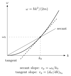
For $\omega=\hbar k^2/(2m)$, the line from the origin has slope $v_p=\omega/k=\hbar k/(2m)$; the tangent has slope $v_g=d\omega/dk=\hbar k/m$. The packet velocity is twice the phase velocity with this energy zero. Axes are schematic.

Schrödinger Equation

For a single spinless nonrelativistic particle in a scalar potential, the coordinate-space equation is

$$i\hbar \frac{\partial}{\partial t} \psi(\mathbf r,t) = \left[ - \frac{\hbar^2}{2m}\nabla^2 + V(\mathbf r,t) \right] \psi(\mathbf r,t).$$

The free-particle part encodes the matter-wave dispersion. The local scalar potential acts by multiplication. This model excludes a vector potential, spin couplings, and relativistic particle creation; those require additional terms or a different theory. Adding the potential is a further physical assumption, not a conclusion from free waves alone.

In modern language, this is a representation of the abstract state equation

$$i\hbar \frac{d}{dt} \lvert\psi(t)\rangle = H\lvert\psi(t)\rangle.$$

The Hamiltonian is the generator of time evolution. In coordinate representation for a particle with scalar potential, it becomes a differential operator. This representation-level distinction matters: the Schrödinger equation is not only a rule for waves in ordinary space; it is the time-evolution law for quantum states represented in a chosen basis.

Stationary States and Spectra

When the Hamiltonian is time independent, one looks for stationary states:

$$H\varphi_n = E_n\varphi_n.$$

The time dependence is then

$$\psi_n(\mathbf r,t) = \varphi_n(\mathbf r) e^{-iE_n t/\hbar}.$$

This is the bridge from wave mechanics to spectra. Bound-state boundary conditions can make only certain energies possible. Hydrogen is the historical example: solving the Coulomb problem gives the Rydberg pattern without classical electron orbits.

The same equation also allows continuum states, scattering states, and wave packets. Therefore the lesson is not “Schrödinger’s equation makes every energy discrete.” The lesson is that spectra follow from the Hamiltonian, boundary conditions, and domain.

To solve a problem, first specify its Hamiltonian and boundary conditions. For moving packets, continue with Free Particle; for allowed bound energies, continue with Time-Independent Schrödinger Equation. In either case, interpreting the solution as outcome probabilities additionally uses the Born rule.

Exercises

1. Show that the free plane wave $Ae^{i(kx-\omega t)}$ satisfies the free Schrödinger equation only if $\omega=\hbar k^2/(2m)$.

Solution

For the plane wave,

$$i\hbar\partial_t\psi = \hbar\omega\psi,$$

and

$$- \frac{\hbar^2}{2m} \partial_x^2\psi = \frac{\hbar^2k^2}{2m}\psi.$$

The equation holds when the coefficients match:

$$\hbar\omega = \frac{\hbar^2k^2}{2m},$$

so

$$\omega = \frac{\hbar k^2}{2m}.$$

2. Use $\omega(k)=\hbar k^2/(2m)$ to compute the group velocity.

Solution

The group velocity is

$$v_g = \frac{d\omega}{dk} = \frac{\hbar k}{m}.$$

Since $p=\hbar k$, this is

$$v_g = \frac{p}{m},$$

the classical nonrelativistic velocity.

3. Why does adding $V(\mathbf r)$ to the Hamiltonian not follow from the free plane-wave argument alone?

Solution

The plane-wave argument uses the free-particle relation $E=p^2/(2m)$. A potential changes the energy function and may introduce position dependence, boundary conditions, and domain issues. Writing $H=p^2/(2m)+V$ and replacing $p$ by $-i\hbar\nabla$ is a successful quantization rule in many nonrelativistic settings, but it is an additional structural step, not a consequence of one free plane wave.

4. Why is the Schrödinger equation not the whole quantum formalism?

Solution

It gives time evolution for a state under a Hamiltonian. The full formalism also needs a state space, observables, probability rules, measurement modeling, composition rules for multiple systems, spin degrees of freedom, and treatment of identical particles and mixed states.

References

• O. Darrigol, From c-Numbers to q-Numbers: The Classical Analogy in the History of Quantum Theory, University of California Press, 1992.
• L. de Broglie, Recherches sur la théorie des quanta, doctoral thesis, Paris, 1924.
• M. Jammer, The Conceptual Development of Quantum Mechanics, 2nd ed., American Institute of Physics, 1989.
• E. Schrödinger, “Quantisierung als Eigenwertproblem,” Annalen der Physik 79, 361-376, 1926.
• E. Schrödinger, “An Undulatory Theory of the Mechanics of Atoms and Molecules,” Physical Review 28, 1049-1070, 1926, DOI: 10.1103/PhysRev.28.1049.
• R. Shankar, Principles of Quantum Mechanics, 2nd ed., Springer, 1994.