Finite-Element Methods

Finite-element methods approximate wavefunctions by locally supported functions and impose the Schrödinger equation in an integrated weak form. They accommodate nonuniform meshes and irregular geometry while retaining a variational structure. The resulting eigenproblem includes an overlap matrix; its coefficient vectors are not normalized by an ordinary unweighted dot product.

Required background. Basis choice explains generalized eigenproblems; Rayleigh–Ritz supplies the variational principle; boundary implementation fixes the domain.

Weak Schrödinger form

For $H=-\alpha\partial_x^2+V(x)$ on $(a,b)$, $\alpha=\hbar^2/(2m)$, consider homogeneous Dirichlet conditions. Multiplying by a test function $v^*$ and integrating by parts gives

$$\alpha\int_a^b v'^*u'\,dx +\int_a^b v^*Vu\,dx =E\int_a^b v^*u\,dx.$$

The test and trial functions vanish at the endpoints, so the boundary term is zero. Only first derivatives are required in the kinetic integral. This permits continuous piecewise-linear functions whose second derivatives are not ordinary functions at mesh nodes.

Expand $u_h=\sum_j c_j\phi_j$ in a finite conforming basis. Testing against each $\phi_i$ gives

$$(K+V_h)c=EMc,$$

where $K_{ij}=\alpha\int\phi_i'^*\phi_j'$, $(V_h)_{ij}=\int\phi_i^*V\phi_j$, and $M_{ij}=\int\phi_i^*\phi_j$. The norm is $c^\dagger Mc=1$. Here “mass matrix” is conventional finite-element terminology for $M$; it is not the particle mass $m$.

Linear elements and assembly

A nodal hat function $\phi_j$ is one at $x_j$, zero at all other nodes, and linear between adjacent nodes. It vanishes outside $[x_{j-1},x_{j+1}]$. Consequently $u_h=\sum_jc_j\phi_j$ interpolates the nodal values $c_j$, while only neighboring hats overlap. This locality makes the assembled matrices sparse.

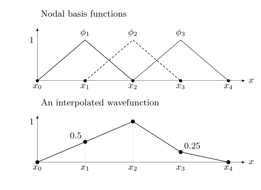
Each hat selects one nodal value. The lower curve is $u_h=0.5\phi_1+\phi_2+0.25\phi_3$ with zero endpoint values. It is continuous, although its derivative jumps at the nodes; the weak form uses its piecewise first derivative.

On one element $[x_e,x_{e+1}]$ of length $h_e$, the two nonzero basis functions restrict to $(x_{e+1}-x)/h_e$ and $(x-x_e)/h_e$. Integrating their products and derivative products gives the local matrices

$$K^{(e)}=\frac{\alpha}{h_e} \begin{pmatrix}1&-1\\-1&1\end{pmatrix}, \qquad M^{(e)}=\frac{h_e}{6} \begin{pmatrix}2&1\\1&2\end{pmatrix}.$$

Add each local contribution into the global rows and columns associated with its two nodes. For a constant potential on an element, $V_h^{(e)}=V_eM^{(e)}$. Otherwise evaluate its weighted integral with a quadrature accurate enough for the chosen basis and potential.

Eliminate endpoint degrees of freedom for Dirichlet conditions. Homogeneous Neumann conditions arise naturally from the vanished boundary flux term when endpoint test values are allowed; nonzero Neumann or Robin data contribute boundary terms. Do not impose a Dirichlet row after deriving a different weak problem.

A variational square-well benchmark

For a uniform mesh with zero potential, the assembled interior matrices have $K_{jj}=2\alpha/h$, $K_{j,j+1}=-\alpha/h$, $M_{jj}=2h/3$, and $M_{j,j+1}=h/6$. Sine vectors diagonalize both, giving

$$E_n^{(h)}= \frac{6\alpha(1-\cos\theta_n)}{h^2(2+\cos\theta_n)}, \qquad \theta_n=\frac{n\pi}{N+1}.$$

For fixed $k_n=n\pi/L$,

$$E_n^{(h)}=\alpha k_n^2 +\frac{\alpha k_n^4h^2}{12}+O(h^4).$$

These eigenvalues approach from above, unlike the centered finite-difference values. For the coarsest mesh with one interior midpoint and two elements of length $L/2$, the energy is $12\alpha/L^2$, above the exact $\pi^2\alpha/L^2$.

The upper-bound property requires a conforming subspace of a semibounded self-adjoint problem and exact evaluation of its quadratic form. Approximate quadrature, mass lumping, or a nonconforming space can change that conclusion. Nested conforming refinements give monotone variational improvement; unrelated meshes need not yield a monotone sequence even if each result remains an upper bound.

Refinement, singularities, and observables

Mesh refinement reduces element size; polynomial refinement raises the local degree. Use small elements where curvature, interfaces, or singular structure demand them. High polynomial degree is most effective for smooth solutions and does not by itself resolve an incorrectly modeled interface.

Residual-based indicators combine the equation residual within elements with jumps of the approximate derivative or flux across element boundaries. A piecewise-linear function has zero second derivative inside each element but still has nonzero derivative jumps, so inspecting only the interior differential residual misses important error information.

Normalize with $M$ and evaluate observables through their finite-element matrices. Squaring nodal coefficients and summing them without quadrature does not compute continuum probability. For derivative-sensitive quantities, check convergence separately from energy.

Practical checks

Verify local matrices by exact integration on a single element. Check global Hermiticity and positive definiteness of $M$ after constraints. Compare the square-well eigenvalues above, then use a nonuniform mesh to test assembly and overlap handling. Convergence studies should vary both resolution and the outer domain when the physical system is unbounded.

Exercises

On a uniform mesh, replace the consistent mass matrix by row-sum lumping with interior diagonal $h$. What free kinetic eigenvalue formula results, and why does the upper-bound argument need reconsideration?

Solution

The eigenvalues become $2\alpha(1-\cos\theta)/h^2=4\alpha\sin^2(\theta/2)/h^2$, the centered finite-difference formula. The inner product has been approximated; this is no longer the exact conforming Rayleigh quotient, and its low-mode energies approach from below. Boundary lumping must be defined before eliminating constrained nodes to obtain the stated interior weights.

References

• Babuška, I., and J. Osborn, “Eigenvalue Problems,” in P. G. Ciarlet and J. L. Lions, eds., Handbook of Numerical Analysis, vol. II, North-Holland, 1991, pp. 641–787 — finite-element spectral approximation.
• Brenner, S. C., and L. R. Scott, The Mathematical Theory of Finite Element Methods, 3rd ed., Springer, 2008 — weak forms, conforming spaces, and error estimates.
• LeVeque, R. J., Finite Difference Methods for Ordinary and Partial Differential Equations, SIAM, 2007 — comparison with finite-difference discretizations.