Convergence Studies

A convergence study measures how a reported observable changes as numerical approximations are systematically reduced. Agreement between two runs tests only the parameters actually changed. Two finely solved matrices in the same undersized box can agree closely and still approximate the wrong physical problem.

Required background. Numerical error and stability distinguishes residuals from physical accuracy; numerical units fixes the scales of tolerances.

Write a computed observable schematically as $Q(h,L,\Delta t,N_b,\varepsilon_s,M)$ , where $h$ is a spatial spacing, $L$ a domain size, $\Delta t$ a time step, $N_b$ a basis cutoff, $\varepsilon_s$ a solver tolerance, and $M$ a sample count. Not every calculation has every parameter. Identify the ones it does have before interpreting an apparent plateau.

For a grid bound-state calculation, first tighten the eigensolver until its error is negligible compared with the differences under study. Refine $h$ at fixed physical $L$ . Then enlarge $L$ while keeping $h$ sufficiently small. Finally revisit the joint limit to check that the two trends do not change materially. Increasing the number of grid points at fixed spacing enlarges the box; it is not a grid-refinement experiment.

Choose observables before running the study. Ground-state energy, tunneling splitting, contact density, and a high-momentum tail can converge at different rates. Monitor all quantities on which the scientific conclusion depends.

Observed order and Richardson extrapolation

Suppose a deterministic sequence enters a regime

Q(h)=Q_*+a h^p+O(h^{p+q}),\qquad p,q>0.

For a fixed refinement factor $r>1$ , three runs estimate

p_{\mathrm{obs}}= \frac{\log\left|\dfrac{Q(h)-Q(h/r)}{Q(h/r)-Q(h/r^2)}\right|}{\log r}.

This estimate is meaningful only if the differences exceed roundoff and solver noise and are dominated by one leading power. When an expected order $p$ is supported by several refinements, the extrapolated value is

Q_{\mathrm{ext}}= \frac{r^pQ(h/r)-Q(h)}{r^p-1}, \qquad Q_*-Q(h/r)\approx\frac{Q(h/r)-Q(h)}{r^p-1}.

An empirical difference is not automatically a rigorous error bound. Changes of sign, unresolved singularities, nonsmooth potentials, and competing powers can invalidate the assumed asymptotic model. Exponential spectral convergence needs a different fit; forcing every sequence into a power law manufactures an order.

An exactly analyzable grid sequence

For the dimensionless infinite well $H=-\partial_x^2$ on $(0,1)$ , use $N$ interior points, $h=1/(N+1)$ , and the centered three-point stencil. Its first eigenvalue is exactly

E_1(h)=\frac{4}{h^2}\sin^2\!\left(\frac{\pi h}{2}\right) =\pi^2-\frac{\pi^4}{12}h^2+O(h^4).

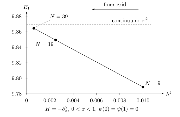
For $h=0.1,0.05,0.025$ , the values are approximately $9.788696741$ , $9.849327524$ , and $9.864532054$ . The observed order from these three points is about $1.996$ . The last two values give the second-order extrapolation $9.869600231$ , close to $\pi^2\approx9.869604401$ .

Three finite-grid ground energies rise toward the continuum energy as the squared grid spacing decreases — The ground energy approaches $\pi^2$ from below. Plotting against $h^2$ makes the leading second-order error nearly linear; the thin segments join the exact discrete eigenvalues for $N=9,19,39$ interior points. An eigensolver can find each dot to high precision without removing its distance from the continuum line.

A generic finite-difference eigenvalue is not a variational upper bound. The extrapolation removes the leading stencil error in this example; reducing the matrix residual alone does not.

State comparisons and statistical sequences

Align a nondegenerate eigenvector’s phase before taking a difference. If $\langle u\vert v\rangle\ne0$ , multiply $v$ by the phase that makes this overlap real and positive. Interpolate different grids into a common physical representation with consistent quadrature. For a nearly degenerate cluster, compare spectral projectors or principal angles between subspaces; individual eigenvectors may rotate freely.

For Monte Carlo estimates, changes across runs contain sampling fluctuation. Plot or report uncertainties alongside means, account for autocorrelation, and use independent repeats or a covariance-aware comparison. A deterministic Richardson formula applied directly to noisy means can give a meaningless order. Systematic time-step bias in stochastic methods should be studied with enough samples to resolve it.

A plateau can indicate convergence, an unvaried dominant approximation, roundoff, an overly loose stopping condition, or a bug that ignores the requested parameter. Record the actual resolved grid and solver iteration count, not only requested inputs. Compare an independent method on a small case and test an analytic limit.

Preserved norm or exact integer topology does not replace refinement: an algorithm can conserve a wrong trajectory, and a coarse topological mesh can produce a stable wrong integer. Convergence reports explains how to present the refinement results and their limits.

Exercises

For a genuinely second-order deterministic method, successive differences are $0.008$ and $0.002$ under halving of $h$ . Estimate the remaining error of the finest result and state the assumption needed.

Solution

The ratio is four, supporting $p=2$ . The leading remaining error magnitude is $0.002/(4-1)\approx0.000667$ . This requires the asymptotic power law to dominate and other errors to be smaller; three values alone cannot prove that condition.

References

LeVeque, R. J., Finite Difference Methods for Ordinary and Partial Differential Equations, SIAM, 2007, publisher edition — consistency, stability, and refinement analysis.
Richardson, L. F., “The Approximate Arithmetical Solution by Finite Differences of Physical Problems Involving Differential Equations, with an Application to the Stresses in a Masonry Dam,” Philosophical Transactions of the Royal Society A 210, 307–357 (1911), original article — extrapolation of discretized solutions.