Alkali Atoms

Neutral alkali atoms are lithium, sodium, potassium, rubidium, caesium, and francium. Each has a closed-shell ionic core and one electron outside it. That architecture makes alkalis the closest many-electron relatives of hydrogen and among the most widely used atoms in spectroscopy, laser cooling, quantum gases, frequency standards, and Rydberg experiments.

The resemblance to hydrogen is powerful but conditional. The valence electron penetrates and polarizes a many-electron core, must be antisymmetrized with core electrons, and experiences spin-dependent and hyperfine interactions. Alkali atoms are therefore not exact one-electron systems. They are systems in which a one-active-electron description is unusually effective and systematically improvable.

Required background. Hydrogenic states and central fields explain orbital labels and screening. Spin–orbit coupling and dipole transitions supply the angular-momentum rules used below.

Closed-Shell Core Plus One Valence Electron

The ground configurations have the form

$$[\text{closed shell}]\,ns,\qquad\text{with term }{}^2S_{1/2}.$$

Examples are $[\mathrm{He}]2s$ for Li, $[\mathrm{Ne}]3s$ for Na, and $[\mathrm{Xe}]6s$ for Cs. Removing the outer electron leaves a positive ion with a closed-shell $^1S_0$ ground state. At low excitation energy, the core often remains in that state while the valence electron changes orbital.

Effective Hamiltonian

In atomic units, a useful schematic Hamiltonian for the active electron is

$$\begin{aligned} H_{\mathrm{val}} &=H_{\mathrm{cf}}+H_{\mathrm{fs}} +H_{\mathrm{hfs}}+H_{\mathrm{ext}},\\ H_{\mathrm{cf}} &=\frac{\mathbf p^2}{2}+V_{\mathrm{core}}(r), \end{aligned}$$

Here a local $V_{\mathrm{core}}$ represents nuclear attraction and screening, with any exchange and correlation effects approximated or fitted. Exact Hartree–Fock exchange is nonlocal and would require an operator in place of this scalar potential. The remaining operators describe fine structure, hyperfine structure, and applied fields.

For a spherical closed-shell ionic core, the leading electrostatic and static dipole-polarization terms far outside it are

$$V_{\mathrm{core}}(r) =-\frac{1}{r}-\frac{\alpha_c}{2r^4} +O(r^{-6}),$$

where $\alpha_c$ is the static dipole polarizability of the singly charged residual ion. The leading $-1/r$ term explains the Rydberg-like spectrum. The polarization term and short-range core structure explain part of the deviation from hydrogen.

What “one valence electron” does not mean

The valence electron is not distinguishable from the core electrons. A proper many-electron state is antisymmetric, and exchange with occupied core orbitals helps enforce orthogonality and changes the effective operator. Nor is the core literally frozen for every observable. It can polarize, participate virtually in transitions, or be excited when the available energy is high enough.

The reduction is most useful below core-excitation thresholds, where core-excited configurations are energetically separated. Strong configuration perturbers, autoionizing resonances, or short-range observables can require an explicit correlated many-electron calculation.

Quantum Defects

An alkali Rydberg series converging to an ionization threshold is organized by

$$E_{n\ell j} =E_{\mathrm{ion}} -\frac{hcR_M}{[n-\delta_{\ell j}(n)]^2},$$

where $R_M$ is the isotope-dependent reduced-mass Rydberg constant in inverse-length units and

$$n^*=n-\delta_{\ell j}(n)$$

is the effective principal quantum number. The quantum defect records the short-range phase shift produced by core penetration, exchange, polarization, and relativistic structure.

Penetration hierarchy

Low-$\ell$ orbitals penetrate the core most strongly and usually have the largest defects. High-$\ell$ Rydberg orbitals are excluded from the core by the centrifugal barrier and become nearly hydrogenic. The qualitative pattern is therefore

$$|\delta_s|,|\delta_p|,|\delta_d| \gg |\delta_f|,|\delta_g|,\ldots$$

for many alkalis, but this is not a numerical law. The ordering and size depend on species, $j$, energy, isotope, and perturbing channels. In heavier alkalis even a $d$ series can retain a substantial defect.

For precision fits, a Ritz expansion is often used:

$$\delta_{\ell j}(n) =\delta_0 +\frac{\delta_2}{(n-\delta_0)^2} +\frac{\delta_4}{(n-\delta_0)^4} +\cdots.$$

The coefficients are empirical or calculated descriptors of one specified series and convention. They should not be moved between isotopes, thresholds, or angular channels without checking the definition and uncertainty.

The same effective quantum number determines the leading binding-energy, orbital-size, and neighboring-level-spacing scalings, developed in Rydberg Atoms Basics.

The Principal Resonance Doublet

The strongest low-lying optical lines connect the ground $nS_{1/2}$ level to the first $nP$ fine-structure pair:

$$\begin{aligned} D_1:&\quad nS_{1/2}\longrightarrow nP_{1/2},\\ D_2:&\quad nS_{1/2}\longrightarrow nP_{3/2}. \end{aligned}$$

These are the alkali D lines. They are electric-dipole allowed because the parity changes and $\Delta J=0,+1$ from a $J=1/2$ ground state. Fine structure separates the two excited levels; hyperfine and Zeeman interactions resolve each nominal line into further components.

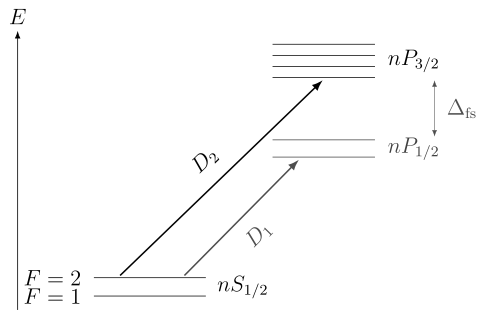
Hierarchy of the alkali resonance doublet, not to scale, illustrated for $I=3/2$ and positive ground-state hyperfine constant $A$. Spin–orbit coupling splits the $nP$ term into $J=1/2$ and $J=3/2$ levels; coupling to the nucleus gives two and four hyperfine levels, respectively. The arrows denote the $D_1$ and $D_2$ optical manifolds. Hyperfine ordering and the number of levels depend on isotope.

Rounded wavelengths and configurations

Element	Ground configuration	Approximate $D_2$ wavelength
Li	$[\mathrm{He}]2s$	$671\ \mathrm{nm}$
Na	$[\mathrm{Ne}]3s$	$589\ \mathrm{nm}$
K	$[\mathrm{Ar}]4s$	$767\ \mathrm{nm}$
Rb	$[\mathrm{Kr}]5s$	$780\ \mathrm{nm}$
Cs	$[\mathrm{Xe}]6s$	$852\ \mathrm{nm}$

All five ground configurations have term $^2S_{1/2}$. These rounded wavelengths locate the resonances; resolving an individual line requires isotope, hyperfine and Zeeman labels, fields, and an air or vacuum convention. Use the NIST Atomic Spectra Database and Steck’s isotope-resolved data for quantitative work.

Fine Structure

In a central-field picture, the leading spin–orbit contribution has the form

$$H_{\mathrm{so}}=\zeta_{n\ell}(r)\,\frac{\mathbf L\cdot\mathbf S}{\hbar^2},$$

where $\zeta$ has units of energy and $\mathbf L,\mathbf S$ are dimensionful angular momenta, or its radial expectation-value reduction within a chosen subshell. For a $P$ state with $L=1$ and $S=1/2$, it gives $J=1/2$ and $J=3/2$. This is the physical origin of the $D_1$–$D_2$ separation at the effective-Hamiltonian level.

The splitting generally becomes larger in heavier alkalis because the valence electron samples stronger relativistic fields. That trend is not captured reliably by inserting a screened charge into the hydrogen fine-structure formula. Core penetration, exchange, correlation, finite nuclear size, and the actual self-consistent radial orbital all matter. Precision fine-structure intervals are many-body atomic-structure observables. Fine Structure develops the relativistic operator hierarchy and the LS, jj, and intermediate-coupling limits.

Hyperfine Structure

If the nucleus has spin $I$, it couples to the electronic angular momentum $J$ to form

$$\mathbf F=\mathbf I+\mathbf J, \qquad F=|I-J|,\ldots,I+J.$$

For a weak magnetic field and a well-resolved fine-structure level, the leading magnetic-dipole constant $A$ gives an energy proportional to $\mathbf I\cdot\mathbf J$. An electric-quadrupole constant $B$ can contribute only when both the nuclear and electronic angular momenta support a rank-2 coupling. Hyperfine Structure derives the $A$–$B$ Hamiltonian, its $F$-dependent spectrum, and the limits of the isolated-$J$ approximation.

Ground-state doublet

For the common alkali isotopes with $I\ne0$, the $nS_{1/2}$ ground state has two hyperfine levels,

$$F=I-\frac12, \qquad F=I+\frac12.$$

Their separation is a microwave frequency. It supplies long-lived internal states for clocks, interferometers, magnetometers, quantum memories, and qubit encodings. “Long lived” does not mean perfectly isolated: magnetic fields, collisions, blackbody radiation, microwave leakage, differential light shifts, and motion can all shift or decohere the transition.

The SI second is defined by fixing the unperturbed ground-state hyperfine transition frequency of caesium-133 to the exact value

$$\Delta\nu_{\mathrm{Cs}} =9\,192\,631\,770\ \mathrm{Hz}.$$

This is a definition of the unit, not the raw frequency of an atom in a laboratory. A caesium primary standard must realize the unperturbed transition by evaluating Zeeman, Stark, collisional, motional, blackbody, cavity, and interrogation shifts with uncertainties.

Magnetic fields and basis changes

In a static field along the quantization axis, $m_F$ remains exact for an axially symmetric Hamiltonian, while $F$ is an approximate label at weak field and the first-order Zeeman shift is approximately

$$\Delta E_Z=g_F\mu_Bm_FB.$$

As the Zeeman energy becomes comparable to the hyperfine splitting, mixing between different $F$ manifolds becomes substantial. The eigenstates continuously approach an uncoupled $|m_I,m_J\rangle$ basis in the hyperfine Paschen–Back regime. Calculations and transition labels must use the coupling scheme appropriate to the field strength; extrapolating a low-field $g_F$ formula through an avoided crossing is not reliable. Zeeman Effect in Atoms develops the Breit–Rabi crossover and its spectroscopic consequences.

Optical Transitions Are Multilevel

At the fine-structure level, an electric-dipole transition changes parity and obeys $\Delta J=0,\pm1$, excluding $J=0\leftrightarrow J'=0$. When hyperfine structure is resolved, the corresponding angular rules include

$$\Delta F=0,\pm1, \qquad F=0\not\leftrightarrow F'=0,$$

and the polarization selects $\Delta m_F=0$ or $\pm1$ relative to the quantization axis. These statements identify angular zeros. Actual line strengths also contain reduced matrix elements, angular coefficients, state mixing, detuning, and experimental polarization geometry.

Cooling and repumping

Many alkali cooling schemes drive a nearly closed component of the $D_2$ manifold. With a suitable quantization axis and circular polarization, a stretched transition can repeatedly absorb and emit photons without immediately changing ground hyperfine level. In practice, off-resonant excitation, imperfect polarization, magnetic-field variation, and unresolved excited-state structure open leakage paths.

If spontaneous emission transfers population into the other ground hyperfine manifold, the cooling light becomes far off resonance and that population is dark. A repump laser returns it to the optical cycle. The need for repumping is not a technical afterthought; it follows directly from the multilevel branching structure.

For an idealized two-level atom, the steady scattering rate is

$$R_{\mathrm{sc}} =\frac{\Gamma}{2} \frac{s}{1+s+(2\Delta/\Gamma)^2},$$

Here $\Gamma=1/\tau$ is the excited-state population decay rate, $\Delta=\omega_L-\omega_0$ is angular-frequency detuning, and $s=2|\Omega|^2/\Gamma^2$ for an interaction $H_{eg}=\hbar\Omega/2$. The weak-drive natural linewidth is $\Gamma$ in angular frequency, or $\Gamma/(2\pi)$ in hertz. The formula assumes a closed transition, a monochromatic steady drive, and no extra dephasing. The mean radiation-pressure force for a single traveling wave is $\hbar\mathbf kR_{\mathrm{sc}}$. In a real alkali atom, Clebsch–Gordan coefficients, optical pumping, several detunings, laser linewidth, and coherences modify the effective rate.

Dark states are sometimes the resource

Coherent superpositions can decouple from the applied light and form dark states. They can reduce an ordinary cooling force, but they also enable sub-Doppler cooling, electromagnetically induced transparency, coherent population trapping, and Raman control. Whether a dark state is an error or a tool depends on the intended effective Hamiltonian and dissipation channels.

From level structure to an experiment

In laser cooling, opposite beams convert Doppler shifts into a velocity-dependent force; a magneto-optical trap adds position-dependent Zeeman shifts. The cooling and repump frequencies must follow the actual isotope’s level structure. Lithium and potassium have comparatively small excited-state hyperfine splittings, so a resolved-level model that works for rubidium need not transfer unchanged.

Ground hyperfine states provide long-lived microwave or Raman transitions. A magnetically insensitive clock transition has zero first derivative of frequency with respect to field at a specified operating point; it generally retains quadratic and other shifts. Raman coupling also introduces light shifts and off-resonant scattering through the eliminated excited levels.

At high principal quantum number, strong Rydberg interactions can prevent simultaneous excitation of nearby atoms. In an isolated van der Waals channel with $V(R)=C_6/R^6$, comparing $|V|$ with $\hbar|\Omega|$ gives the estimate $R_b=(|C_6|/\hbar|\Omega|)^{1/6}$. Angular structure, resonant channels, linewidth, and motion limit that estimate.

Different isotopes also supply bosonic and fermionic atoms: $^7$Li is bosonic whereas $^6$Li is fermionic; $^{39}$K is bosonic whereas $^{40}$K is fermionic. Electronic valence structure alone does not fix atomic statistics or ultracold interactions. Those require nuclear spin and multichannel molecular scattering as well.

Exercises

1. Residual-core potential

A valence electron is at radius $r$ outside the closed-shell core of a neutral alkali atom. Use charge counting to derive the leading Coulomb potential. If the core polarizability is $\alpha_c$, find the radius at which the magnitudes of the formal terms $-1/r$ and $-\alpha_c/(2r^4)$ are equal. Why should that radius be interpreted cautiously?

Solution

If the neutral atom has nuclear charge $Z$ and $Z$ electrons, the core contains $Z-1$ electrons. Its net charge is therefore

$$Z-(Z-1)=+1.$$

The distant valence electron has potential energy $-1/r$ in atomic units. Equating the magnitudes of the Coulomb and polarization terms gives

$$\frac1r=\frac{\alpha_c}{2r^4}, \qquad r=\left(\frac{\alpha_c}{2}\right)^{1/3}.$$

This is only a comparison of asymptotic terms. If the resulting radius lies in or near the electronic core, the multipole and polarization expansion is not quantitatively valid there. Exchange, penetration, finite core size, and higher response terms then require a microscopic or fitted potential.

2. Hyperfine doublet and centroid

Consider an alkali $S_{1/2}$ level in an isotope with $I=3/2$. List the allowed $F$ values. Using only the magnetic-dipole term $E_F=AK/2$, find both energies relative to the hyperfine center of gravity and show that their separation is $2A$.

Solution

With $I=3/2$ and $J=1/2$,

$$F=|I-J|,I+J=1,2.$$

The quantity $K$ is

$$\begin{aligned} K_{F=2} &=2(3)-\frac32\frac52-\frac12\frac32 =\frac32,\\ K_{F=1} &=1(2)-\frac32\frac52-\frac12\frac32 =-\frac52. \end{aligned}$$

Hence

$$E_2=\frac{3A}{4}, \qquad E_1=-\frac{5A}{4},$$

and $E_2-E_1=2A$. The degeneracy-weighted centroid vanishes:

$$\frac{(2\cdot2+1)E_2+(2\cdot1+1)E_1}{5+3}=0.$$

This confirms that the quoted energies are measured from the unresolved fine-structure level’s center of gravity. The electric-quadrupole term vanishes because $J=1/2$.

3. Why there are two D lines

Use angular momentum and parity to explain why an alkali $nS_{1/2}$ ground state has allowed transitions to both $nP_{1/2}$ and $nP_{3/2}$. Why does this not imply that each D line is an isolated two-level transition?

Solution

For the ground state, $L=0$ and $S=1/2$, so $J=1/2$. The excited $P$ term has $L=1$ and $S=1/2$, which can couple to

$$J=\left|L-S\right|,L+S =\frac12,\frac32.$$

An electric-dipole operator changes parity and allows $\Delta J=0,\pm1$ except $0\leftrightarrow0$. Both $1/2\to1/2$ and $1/2\to3/2$ therefore survive, giving $D_1$ and $D_2$.

If $I\ne0$, each fine-structure level contains several $F$ levels and each $F$ contains $2F+1$ magnetic sublevels. Polarization, Zeeman shifts, and spontaneous-emission branching connect different subsets. The “D line” is consequently a manifold, and a two-level reduction requires specified detuning, polarization, fields, and leakage bounds.

4. Binding from illustrative quantum defects

Two Rydberg series converge to the same threshold. At $n=20$, take the illustrative defects $\delta_s=3.13$ and $\delta_f=0.02$. Find the effective principal quantum numbers and the ratio of binding-energy magnitudes in the constant-defect approximation.

Solution

The effective quantum numbers are

$$\begin{aligned} n_s^*&=20-3.13=16.87,\\ n_f^*&=20-0.02=19.98. \end{aligned}$$

Because the binding magnitude scales as $(n^*)^{-2}$,

$$\frac{|E_s-E_{\mathrm{ion}}|} {|E_f-E_{\mathrm{ion}}|} =\left(\frac{19.98}{16.87}\right)^2 \approx1.40.$$

The more strongly penetrating $s$ state is about $40\%$ more deeply bound at the same nominal $n$ in this model. The defects here are illustrative inputs, not universal alkali constants; a precision calculation would use a specified series fit and its energy dependence.

5. Why a repump is needed

A cooling laser addresses a ground hyperfine level $F=2$. The desired cycling transition reaches $F'=3$, which can decay only back to $F=2$ under the electric-dipole $\Delta F$ rule. Explain why population can nevertheless accumulate in a second ground level $F=1$, and describe the role of a repump laser.

Solution

The ideal $F=2\to F'=3$ branch is closed with respect to hyperfine decay because $F'=3\to F=1$ would have $\Delta F=-2$. Real cooling light can also excite nearby $F'=2$ through finite detuning, power broadening, imperfect polarization, or unresolved structure. That level may decay to either $F=2$ or $F=1$.

Once an atom reaches $F=1$, the cooling laser is displaced by approximately the ground hyperfine splitting and scatters very weakly. The atom becomes dark to the cooling cycle. A repump laser drives $F=1$ to an excited level that can decay into $F=2$, restoring population to the cycle. A quantitative model must include the relevant branching ratios and coherences rather than assigning a perfect closure by label alone.

References

• E. Arimondo, M. Inguscio, and P. Violino, “Experimental Determinations of the Hyperfine Structure in the Alkali Atoms,” Reviews of Modern Physics 49, 31–75 (1977), doi:10.1103/RevModPhys.49.31.
• A. Browaeys and T. Lahaye, “Many-Body Physics with Individually Controlled Rydberg Atoms,” Nature Physics 16, 132–142 (2020), doi:10.1038/s41567-019-0733-z.
• Bureau International des Poids et Mesures, SI Base Unit: Second and The International System of Units, 9th ed.
• C. J. Foot, Atomic Physics (Oxford University Press, 2005), Chapters 4–9.
• T. F. Gallagher, Rydberg Atoms (Cambridge University Press, 1994), doi:10.1017/CBO9780511524530.
• W. R. Johnson, Atomic Structure Theory: Lectures on Atomic Physics (Springer, 2007), doi:10.1007/978-3-540-68013-0.
• A. Kramida, Y. Ralchenko, J. Reader, and the NIST ASD Team, NIST Atomic Spectra Database, National Institute of Standards and Technology, doi:10.18434/T4W30F.
• H. J. Metcalf and P. van der Straten, Laser Cooling and Trapping (Springer, 1999), doi:10.1007/978-1-4612-1470-0.
• National Institute of Standards and Technology, Atomic Spectroscopy: Term Series and Quantum Defects.
• National Institute of Standards and Technology, Basic Atomic Spectroscopic Data: Li, Na, K, Rb, and Cs, with associated persistent- and strong-line tables.
• E. L. Raab, M. Prentiss, A. Cable, S. Chu, and D. E. Pritchard, “Trapping of Neutral Sodium Atoms with Radiation Pressure,” Physical Review Letters 59, 2631–2634 (1987), doi:10.1103/PhysRevLett.59.2631.
• M. Saffman, T. G. Walker, and K. Mølmer, “Quantum Information with Rydberg Atoms,” Reviews of Modern Physics 82, 2313–2363 (2010), doi:10.1103/RevModPhys.82.2313.
• D. A. Steck, Alkali D Line Data, isotope-resolved reference sheets, revision 2.3.4 (8 August 2025), accessed 13 October 2026.