Time Ordering

Time ordering arranges products of time-labeled operators so that later times appear to the left. It is required when Hamiltonians or interaction operators at different times do not commute.

Chronological operator products

For ordinary operators, or even-parity field operators, at distinct times,

$$\mathcal T[A(t_1)B(t_2)] = \begin{cases} A(t_1)B(t_2), & t_1\gt t_2,\\ B(t_2)A(t_1), & t_2\gt t_1. \end{cases}$$

For more operators, $\mathcal T$ orders the product with the latest time on the left and the earliest time on the right. In a product acting on a ket, the rightmost factor acts first. Time ordering of fermionic field insertions additionally includes a minus sign for each exchange; that graded convention is separate from the Hamiltonian evolution considered here. Equal-time products need a stated prescription when operator distributions or contact terms are involved.

Why It Appears

Time evolution is a product of short-time steps. For a time-dependent Hamiltonian,

$$U(t+\Delta t,t) \approx I-\frac{i}{\hbar}H(t)\Delta t.$$

Multiplying many such factors gives later time steps on the left because they act after earlier time steps. If the Hamiltonians do not commute, this order cannot be rearranged.

Time-Ordered Exponential

For forward evolution, $t\ge t_0$, the compact notation is

$$U(t,t_0) = \mathcal T \exp\left[ -\frac{i}{\hbar} \int_{t_0}^{t}H(t')\,dt' \right].$$

This is shorthand for a series with ordered operator products. If $[H(s),H(s')]=0$ throughout the interval, it becomes the ordinary exponential of the integrated Hamiltonian. Backward evolution is the inverse: $U(t_0,t)=\overline{\mathcal T}\exp[+(i/\hbar)\int_{t_0}^tH(s)\,ds]$, with earlier factors on the left. Here $\overline{\mathcal T}$ denotes anti-time ordering.

Dyson Series

The time-ordered exponential expands as

$$U(t,t_0) =I +\left(-\frac{i}{\hbar}\right) \int_{t_0}^{t}dt_1\,H(t_1) +\cdots.$$

The second-order term is

$$\left(-\frac{i}{\hbar}\right)^2 \int_{t_0}^{t}dt_1 \int_{t_0}^{t_1}dt_2\, H(t_1)H(t_2).$$

The ordered integration region $t_1\gt t_2$ is what enforces the operator order.

Two pulses with different outcomes

Let $U_x=e^{-i\pi\sigma_x/4}$ and $U_z=e^{-i\pi\sigma_z/4}$ be positive quarter-turns of a spin’s Bloch vector. Starting from the $+1$ eigenstate $\lvert0\rangle$ of $\sigma_z$, an $x$ pulse followed by a $z$ pulse gives

$$U_zU_x\lvert0\rangle=e^{-i\pi/4}\lvert+_x\rangle.$$

Reversing the order gives

$$U_xU_z\lvert0\rangle=e^{-i\pi/4}\lvert-_y\rangle.$$

The first sequence gives $\sigma_x=+1$ with certainty; the second gives that outcome with probability $1/2$. Time ordering changes a measurable prediction, not merely the appearance of the operator product.

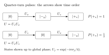
Read the arrows from left to right and the operator product from right to left. The states are shown up to a global phase. Reversing the same two pulses changes $P(+_x)$ from $1$ to $1/2$.

Correlation Functions Preview

Time ordering also appears in correlation functions, such as

$$\langle\psi\rvert \mathcal T[A(t_1)B(t_2)] \lvert\psi\rangle.$$

This notation becomes central in perturbation theory, Green functions, and field-theory propagators.

From Evolution Operators to Time-Ordered Products explains how this ordering rule governs field insertions, Wick expansions, and scattering amplitudes.

Common Mistakes

• Treating $\mathcal T$ as decorative notation.
• Pulling noncommuting operators through a time-ordered product.
• Forgetting that time ordering is tied to the order in which operators act.
• Assuming the ordinary exponential of an integral is valid for noncommuting $H(t)$.
• Confusing time ordering with normal ordering, which is a different operation.

References

• A. Altland and B. Simons, Condensed Matter Field Theory, 2nd ed., Cambridge University Press, 2010.
• M. E. Peskin and D. V. Schroeder, An Introduction to Quantum Field Theory, Addison-Wesley, 1995.
• J. J. Sakurai and J. Napolitano, Modern Quantum Mechanics, 3rd ed., Cambridge University Press, 2020.

Exercises

1. Suppose $t_1\gt t_2$. What is $\mathcal T[B(t_2)A(t_1)]$?

Solution

Time ordering places the later-time operator on the left. Since $t_1\gt t_2$,

$$\mathcal T[B(t_2)A(t_1)] =A(t_1)B(t_2).$$

This may differ from the original product if the two operators do not commute.