Tensor-Network Overview

A tensor network replaces a large array by smaller arrays whose repeated indices are summed. Its computational value depends on two separate questions: whether the state or operator admits small internal dimensions, and whether the chosen contraction can be performed without creating large intermediate arrays. This page makes those questions explicit before an algorithm is selected.

Required background. Tensor products in code fixes index ordering; the Schmidt decomposition supplies the rank criterion for an exact factorization. The physical role of entanglement belongs to tensor-network entanglement.

Physical indices, virtual indices, and storage

For $N$ sites of local dimension $d$, a state has coefficients $C_{s_1\ldots s_N}$. A chain factorization uses

$$C_{s_1\ldots s_N} =\sum_{\alpha_1,\ldots,\alpha_{N-1}} A^{[1]s_1}_{1\alpha_1} A^{[2]s_2}_{\alpha_1\alpha_2} \cdots A^{[N]s_N}_{\alpha_{N-1}1}.$$

The $s_j$ are physical indices and $\alpha_j$ are virtual indices. Open boundaries mean $D_0=D_N=1$; the exact storage is $\sum_j dD_{j-1}D_j$. If all internal dimensions are bounded by $D$, this is at most $NdD^2$, instead of $d^N$. This is a storage bound, not a guarantee that a prescribed error can be reached at fixed $D$.

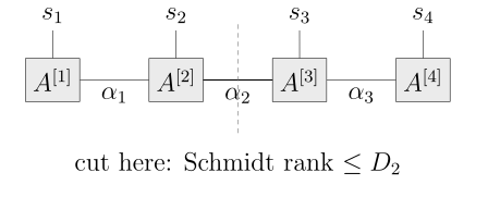
Each box is a small array. An open vertical line labels a physical basis index $s_j$; a joined horizontal line means summation over a shared index $\alpha_j$. At the dashed cut, the two halves communicate through only $D_2$ values of $\alpha_2$, so the Schmidt rank cannot exceed $D_2$. The end bonds have dimension one and are omitted.

Repeated SVDs construct such a factorization for every finite state, but generic middle bonds require $D\sim d^{N/2}$. Compression is therefore a property of the state and its ordering, not of the notation.

A contraction is an algorithm

Consider $X_{ab}Y_{bc}Z_{cd}$ with dimensions $a,c=\chi$ and $b,d=d$. Computing $(XY)Z$ costs approximately $\chi^2d+\chi^2d$, whereas $X(YZ)$ costs approximately $\chi d^2+\chi d^2$. When $\chi\gg d$, the latter saves both arithmetic and intermediate memory. This elementary example explains why a drawing of the same network does not specify its runtime.

For an MPS norm, contract a left environment rather than constructing $C$:

$$L_j=\sum_{s_j}(A^{[j]s_j})^\dagger L_{j-1}A^{[j]s_j}, \qquad L_0=1.$$

The final scalar is $\langle\psi|\psi\rangle$. With bounded dimensions, this costs $O(NdD^3)$. In left-canonical gauge, each intermediate $L_j=I$, providing a useful implementation invariant.

An exact small-network benchmark

A product state has $A^{[j]s}=v_j^s$ and $D=1$. A chain of $N$ qubits therefore requires $2N$ complex numbers before exploiting normalization. For the normalized GHZ state, $(|0\cdots0\rangle+|1\cdots1\rangle)/\sqrt2$, $D=2$ suffices across every internal cut. These examples test very different behavior: both compress well, but GHZ has nonzero long-distance connected correlations.

On four sites, explicitly reconstruct all $16$ coefficients and compare the norm and one-site and two-site expectations with direct dense contractions. To test site ordering, use an asymmetric complex state and deliberately permute two physical axes: site-resolved observables should change while the norm stays fixed. The GHZ state is invariant under site permutations and therefore cannot reveal this mistake by itself.

Choosing the approximation

Use MPS for chain factorizations, MPOs for operator structure, and PEPS when two-dimensional connectivity matters. A circuit contraction can be exact but expensive; an MPS simulation of the same circuit can be cheaper and approximate.

Record the maximum intermediate size, bond dimensions, contraction order, and every truncation. Changes in contraction order should agree to roundoff when no compression occurs. Changes in bond dimension probe representation error. These are different tests.

Exercises

A normalized state has Schmidt weights $0.8,0.15,0.05$ across one cut. What fidelity is obtained by retaining two terms and renormalizing?

Solution

The retained squared norm is $0.95$. The overlap with the normalized retained state is $\sqrt{0.95}$, so the squared fidelity is $0.95$. A different tensor gauge cannot improve this rank-two optimum for that cut. Multiple successive cuts require a separate accumulated-error analysis.

References

• Orús, Román, “A practical introduction to tensor networks: Matrix product states and projected entangled pair states,” Annals of Physics 349, 117–158 (2014), arXiv:1306.2164 — representations and approximate contractions.
• Schollwöck, Ulrich, “The density-matrix renormalization group in the age of matrix product states,” Annals of Physics 326, 96–192 (2011), arXiv:1008.3477 — canonical gauges, contractions, and finite-chain algorithms.