Entanglement Entropy

Entanglement entropy quantifies bipartite pure-state entanglement through the mixedness of either subsystem. Throughout the finite-dimensional discussion, logarithms are base two and entropy is measured in bits. If the joint state on $AB$ is pure,

$$\rho_{AB} = \lvert\Psi\rangle\langle\Psi\rvert,$$

then the entanglement entropy across the $A\vert B$ split is

$$S_A = S(\rho_A) = -\operatorname{Tr}(\rho_A\log_2\rho_A), \qquad \rho_A=\operatorname{Tr}_B\rho_{AB}.$$

For pure bipartite states, this quantity measures how entangled $A$ is with $B$. For mixed joint states, the entropy of a subsystem is not by itself an entanglement measure.

Helpful background. Schmidt decomposition gives the reduced-state spectrum; subsystem entropy distinguishes state entropy from measurement uncertainty.

Entanglement entropy of a pure bipartite state

Let

$$\lvert\Psi\rangle_{AB} \in \mathcal H_A\otimes\mathcal H_B$$

be a normalized pure state. Define

$$\rho_A=\operatorname{Tr}_B \bigl( \lvert\Psi\rangle\langle\Psi\rvert \bigr), \qquad \rho_B=\operatorname{Tr}_A \bigl( \lvert\Psi\rangle\langle\Psi\rvert \bigr).$$

The entanglement entropy is

$$E(\Psi) = S(\rho_A) = S(\rho_B).$$

The equality $S(\rho_A)=S(\rho_B)$ holds because the nonzero spectra of $\rho_A$ and $\rho_B$ are the same for a pure bipartite state.

Computing entropy from Schmidt probabilities

Write $|\Psi\rangle=\sum_r s_r|u_r\rangle_A|v_r\rangle_B$ and let $p_r=s_r^2$. Both reduced states have the same nonzero eigenvalues $p_r$, so

$$E(\Psi)=S(\rho_A)=S(\rho_B)=-\sum_r p_r\log_2 p_r.$$

Use $0\log_2 0=0$, understood by continuity. This is the Shannon entropy of the squared Schmidt coefficients, not the coefficients themselves. Natural-logarithm entropy is obtained by multiplying the value in bits by $\ln2$.

For Schmidt probabilities $(0.9,0.1)$, the entropy is $-0.9\log_2 0.9-0.1\log_2 0.1\simeq0.469$ bits. A Bell pair has $(1/2,1/2)$ and one bit, conventionally called one ebit of entanglement. A product vector has the single probability $1$ and zero entropy.

Partially Entangled Two-Qubit State

For

$$\lvert\Psi_\theta\rangle = \cos\theta\,\lvert00\rangle + \sin\theta\,\lvert11\rangle, \qquad 0\le\theta\le\frac{\pi}{2},$$

the Schmidt probabilities are

$$p_1=\cos^2\theta, \qquad p_2=\sin^2\theta.$$

The entanglement entropy in bits is

$$E_2(\Psi_\theta) = -\cos^2\theta\,\log_2(\cos^2\theta) -\sin^2\theta\,\log_2(\sin^2\theta).$$

It is zero at $\theta=0$ and $\theta=\pi/2$, and it reaches one bit at $\theta=\pi/4$.

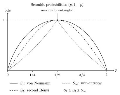
The same two Schmidt probabilities give different spectral entropies. All three vanish for a product state and equal one bit at $p=1/2$; between those limits, larger Rényi order emphasizes the larger probability. The curves describe pure joint states when interpreted as entanglement.

Maximum Value

If the smaller subsystem dimension is

$$d=\min(\dim\mathcal H_A,\dim\mathcal H_B),$$

then

$$0\le E_2(\Psi)\le \log_2 d.$$

Zero entropy occurs exactly for a product vector. For the upper bound, compare the Schmidt probability vector (padded with zeros to length $d$) with the uniform vector. Nonnegativity of classical relative entropy gives $0\le\sum_r p_r\log_2(dp_r)=\log_2d-E$. Equality holds exactly for the uniform probabilities:

$$p_r=\frac1d, \qquad r=1,\ldots,d.$$

Then

$$E_2(\Psi)=\log_2 d.$$

For two qubits, this maximum is $1$ bit. For two qutrits, it is $\log_2 3$ bits.

What local measurements can change

For a local measurement resolved into one Kraus operator per recorded branch $m$, a pure input gives pure branch states with probabilities $q_m$ and remote reduced states $\rho_B^{(m)}$. If the measurement is complete, no signaling gives $\sum_m q_m\rho_B^{(m)}=\rho_B$. Concavity of von Neumann entropy then implies

$$\sum_m q_m E(\Psi_m) =\sum_m q_m S(\rho_B^{(m)}) \le S(\rho_B)=E(\Psi).$$

A successful postselected branch may have more entanglement, but the average over all outcomes cannot increase under LOCC. For example, the local filter in Schmidt rank turns probabilities $(0.9,0.1)$ into a Bell pair with probability $0.2$, while failure produces a product state. The output average is $0.2$ ebits, below the input’s $0.469$.

This entropy also has an operational asymptotic meaning: many independent identical copies of a known finite-dimensional pure state can be reversibly converted into Bell pairs by LOCC at a rate $E(\Psi)$ per copy, with error vanishing as the number of copies grows (Bennett et al.). This does not promise an exact deterministic conversion of one copy into a fractional Bell pair.

What It Measures and What It Does Not

For a pure bipartite state, entanglement entropy measures the amount of entanglement across the chosen split. It is invariant under local unitaries:

$$\lvert\Psi\rangle \mapsto (U_A\otimes U_B)\lvert\Psi\rangle.$$

It is also additive for independent pure pairs:

$$E(\Psi_1\otimes\Psi_2) = E(\Psi_1)+E(\Psi_2).$$

Here the combined partition is $A_1A_2:B_1B_2$. Additivity follows because the combined Schmidt probabilities are all products $p_rq_s$.

However, $S(\rho_A)$ is not a general mixed-state entanglement measure. If $\rho_{AB}$ is mixed, subsystem entropy can include ordinary classical uncertainty, thermal entropy, environmental noise, and correlations that are not entanglement. Mixed-state entanglement requires different tools.

Many-Body and QFT Preview

In many-body physics, one often studies the entropy of a spatial region or a collection of sites in a pure many-body state. The same formula appears:

$$S_A=-\operatorname{Tr}(\rho_A\log_2\rho_A).$$

The interpretation becomes richer. Entanglement entropy can diagnose area laws, critical scaling, topological order, tensor-network efficiency, and thermalization behavior.

In QFT, entanglement entropy is subtle because local regions have infinitely many degrees of freedom. The entropy often depends on a short-distance regulator and can diverge. The finite-dimensional formula here is the conceptual starting point, not the complete field-theoretic story.

For spatial partitions, exact many-body benchmarks, area and volume laws, critical scaling, and tensor-network consequences, see Entanglement Entropy in Many-Body Systems. For continuum-region, modular-Hamiltonian, relative-entropy, and holography cautions, see Entanglement in QFT Preview.

Limits of the entropy description

Entropy is a nonlinear function of the state, not the expectation value of one fixed single-copy observable. Its estimation therefore requires a specified protocol and enough information about the state.

For normalizable infinite-dimensional pure states the two reduced spectra still agree, but their common entropy may be infinite. Without an energy constraint there need not be a finite maximum; the finite-dimensional $\log_2d$ bound cannot simply be reused.

References

• C. H. Bennett, H. J. Bernstein, S. Popescu, and B. Schumacher, “Concentrating partial entanglement by local operations”, Physical Review A 53, 2046–2052 (1996).
• J. Eisert, M. Cramer, and M. B. Plenio, “Area laws for the entanglement entropy”, Reviews of Modern Physics 82, 277–306 (2010).
• M. A. Nielsen and I. L. Chuang, Quantum Computation and Quantum Information, 10th anniversary ed., Cambridge University Press (2010).
• J. Watrous, The Theory of Quantum Information, Cambridge University Press (2018), Chs. 5 and 6.

Exercises

1. A pure two-qutrit state has Schmidt probabilities $(2/3,1/6,1/6)$. Compute its entropy and compare it with the maximum.

Solution

$E=-\tfrac23\log_2(2/3)-\tfrac13\log_2(1/6)=\log_2 3-\tfrac13\simeq1.252$ bits. The maximum is $\log_2 3\simeq1.585$ bits. Full rank does not imply maximal entropy.

2. Compute the entanglement entropy in bits of

$$\lvert\Psi\rangle = \frac{1}{\sqrt3} \bigl( \lvert00\rangle+\lvert11\rangle+\lvert22\rangle \bigr).$$

Solution

The Schmidt probabilities are

$$p_1=p_2=p_3=\frac13.$$

Thus

$$E_2 = -3\left(\frac13\log_2\frac13\right) = \log_2 3.$$

3. For Schmidt probabilities $(1-\epsilon,\epsilon)$, show that the entanglement tends continuously to zero as $\epsilon\to0^+$, while Schmidt rank remains two.

Solution

Using $\ln(1-\epsilon)=-\epsilon+O(\epsilon^2)$ gives

$$E=-\epsilon\log_2\epsilon+\frac{\epsilon}{\ln2}+O(\epsilon^2).$$

Both terms tend to zero, but both Schmidt coefficients remain nonzero for every $0<\epsilon<1$. Exact rank detects presence; entropy captures weight.

4. Why is $S(\rho_A)$ not automatically an entanglement measure when $\rho_{AB}$ is mixed?

Solution

If $\rho_{AB}$ is mixed, $\rho_A$ may be mixed because of classical uncertainty, thermal noise, environmental correlations, entanglement, or a combination of these. The entropy of $\rho_A$ does not distinguish these origins. For pure $\rho_{AB}$, a mixed reduced state has only one possible source: entanglement with the other subsystem.