Wave-Mechanics Visualization Gallery

A quantum plot becomes easier to understand when you identify both the plotted quantity and its measure. The examples below contrast density with amplitude, radial shell probability with local density, and a gauge transformation with a change of basis. For a visual tour of the models, see Canonical Plots Gallery.

A Spreading Packet Keeps Its Total Probability

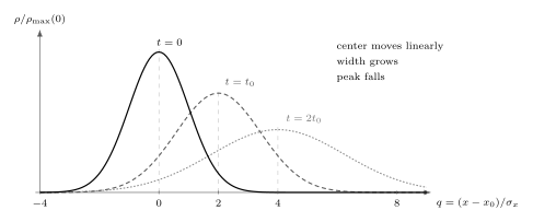
An initially unchirped Gaussian at $t=0,t_0,2t_0$, where $t_0=2m\sigma_x^2/\hbar$. The horizontal coordinate is $(x-x_0)/\sigma_x$, and the density is divided by its initial peak. The center travels two initial widths per $t_0$. The full curves have equal area even though their peak heights differ.

The probability of a region is the area under its density curve. As the packet spreads, a fixed small interval around its center generally contains less probability, while more lies in the tails. A peak height alone does not give the chance of finding the particle in a finite interval. Derive the width in Gaussian Wave Packets.

Radial Probability Includes the Size of a Shell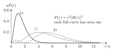

Radial shell probabilities for hydrogenic $1s$, $2s$, and $2p$ states as functions of $r/a$, with $a$ the ionic Bohr length. The vertical axis is the dimensionless density $aP(r)$; each full curve has area one in $r/a$. The $2s$ node is at $r=2a$.

For a normalized angular factor, $P(r)=r^2|R(r)|^2$ is the density with respect to $dr$. The $1s$ local density is greatest at the origin, but the probability per radial interval vanishes there because a shell has vanishing volume. Its maximum occurs at $r=a$. The distinction is developed in Radial Probability Distributions.

Gauge Changes and Basis Changes

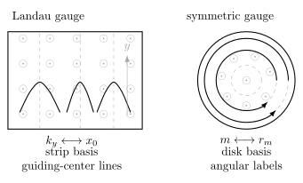
Two convenient bases for the same ideal bulk Landau-level problem: translation-adapted states labeled by a guiding center, and rotation-adapted states labeled by angular momentum. The outlines illustrate coordinate regions rather than imposed hard boundaries; arrows are schematic labels, not particle trajectories.

A gauge transformation multiplies the wavefunction of the same state by a phase and leaves $|\psi|^2$ unchanged. The different shapes here arise because one also chooses different basis states within a degenerate energy eigenspace. To compare the same state across gauges, transform the whole state, including the appropriate superposition coefficients. See Landau Gauge vs Symmetric Gauge.

Exercises

1. Can a negative part of a plotted wavefunction represent a negative probability?

Solution

No. A real amplitude can change sign, and a complex amplitude has a phase. Probability density is its nonnegative modulus squared. Opposite signs still matter when amplitudes interfere.

2. A normalized Gaussian has twice its original width. What happens to its peak density?

Solution

For $\rho(x)=e^{-(x-\bar x)^2/(2\sigma^2)}/(\sqrt{2\pi}\sigma)$, the peak is $1/(\sqrt{2\pi}\sigma)$. Doubling $\sigma$ halves the peak, preserving total area one.

References

• D. J. Griffiths and D. F. Schroeter, Introduction to Quantum Mechanics, 3rd ed., Cambridge University Press, 2018, chapters 2, 4, and 10.
• R. Shankar, Principles of Quantum Mechanics, 2nd ed., Springer, 1994, chapters 5, 12, and 14.