Bloch Sphere: Wave-Mechanics Perspective

The Bloch sphere is a visualization of normalized pure states in a two-dimensional Hilbert space after global phase has been removed. In this wave-mechanics first encounter, the two basis states may be localized well states, two internal atomic states, two site orbitals, or spin-up and spin-down states. The sphere is not tied to spin until a spin interpretation is added.

Choose an orthonormal basis

$$\{\lvert1\rangle,\lvert2\rangle\}.$$

A normalized pure state is

$$\lvert\psi\rangle =c_1\lvert1\rangle+c_2\lvert2\rangle, \qquad \lvert c_1\rvert^2+\lvert c_2\rvert^2=1.$$

Multiplying the whole state by a common phase does not change the physical ray. After using that freedom, every ray can be represented as

$$\lvert\psi(\theta,\phi)\rangle = \cos\frac{\theta}{2}\,\lvert1\rangle + e^{i\phi}\sin\frac{\theta}{2}\,\lvert2\rangle,$$

with

$$0\leq\theta\leq\pi, \qquad 0\leq\phi\lt 2\pi.$$

The angle $\theta$ records the population imbalance. The angle $\phi$ records the relative phase.

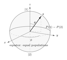
The Bloch sphere represents pure two-level rays. The polar angle fixes the relative populations of $\lvert1\rangle$ and $\lvert2\rangle$, while the azimuthal angle fixes their relative phase.

Helpful background. Two-Level Systems to work with a pair of orthonormal state amplitudes.

From Coefficients To A Sphere

The Bloch vector associated with $\lvert\psi(\theta,\phi)\rangle$ is

$$\mathbf r = (\sin\theta\cos\phi,\, \sin\theta\sin\phi,\, \cos\theta).$$

It has unit length:

$$\lVert\mathbf r\rVert=1.$$

Thus the two real parameters left after normalization and global phase form the surface of a sphere. The north pole is $\lvert1\rangle$, the south pole is $\lvert2\rangle$, and the equator consists of equal-population superpositions.

For example,

$$\frac{\lvert1\rangle+\lvert2\rangle}{\sqrt2}$$

lies on the positive $x$ axis, while

$$\frac{\lvert1\rangle+i\lvert2\rangle}{\sqrt2}$$

lies on the positive $y$ axis. These two states have the same populations in the chosen basis but different relative phases.

Pauli Expectation Values

In the chosen basis, use the standard Pauli matrices. The Bloch-vector components are expectation values:

$$r_i = \langle\psi\vert\sigma_i\vert\psi\rangle, \qquad i=x,y,z.$$

Equivalently, the projector onto the ray is

$$\lvert\psi\rangle\langle\psi\rvert = \frac12 \left( I+\mathbf r\cdot\boldsymbol\sigma \right).$$

This formula is often the cleanest bridge between state-vector language and measurement probabilities. The Bloch vector is not an additional hidden variable; it is the same pure state written in Pauli coordinates.

Population, Phase, And Measurement

Measurement in the displayed basis has probabilities

$$P(1) = \lvert\langle1\vert\psi\rangle\rvert^2 = \cos^2\frac{\theta}{2} = \frac{1+r_z}{2},$$

and

$$P(2) = \lvert\langle2\vert\psi\rangle\rvert^2 = \sin^2\frac{\theta}{2} = \frac{1-r_z}{2}.$$

So the vertical coordinate $r_z$ is a population imbalance:

$$r_z=P(1)-P(2).$$

The azimuthal angle $\phi$ does not affect these two probabilities, but it affects interference and measurements in other bases. That is why relative phase is physically observable even though global phase is not.

More generally, measuring the Pauli component along a unit direction $\hat{\mathbf n}$ uses projectors

$$P_\pm(\hat{\mathbf n}) = \frac12 \left( I\pm\hat{\mathbf n}\cdot\boldsymbol\sigma \right).$$

For a pure state with Bloch vector $\mathbf r$,

$$p_\pm = \frac12 \left( 1\pm\mathbf r\cdot\hat{\mathbf n} \right).$$

The measurement reads the projection of the Bloch vector onto the measurement axis.

Hamiltonian Motion

For a two-level Hamiltonian

$$H=c_0I+\mathbf b\cdot\boldsymbol\sigma,$$

the term $c_0I$ contributes only a global phase. The vector $\mathbf b$ rotates the Bloch vector according to

$$\frac{d\mathbf r}{dt} = \frac{2}{\hbar}\, \mathbf b\times\mathbf r.$$

Thus $\mathbf r$ precesses around the axis $\mathbf b$ with angular frequency

$$\omega_{\mathrm{Bloch}} = \frac{2\lvert\mathbf b\rvert}{\hbar}.$$

This is the geometric version of two-state coherent oscillation. If the state starts away from the Hamiltonian axis, its Bloch vector moves. Probabilities for a measurement along that axis remain constant; probabilities for a transverse measurement generally oscillate. If it starts aligned or anti-aligned with $\mathbf b$, it is an energy eigenstate and the Bloch vector is stationary.

The algebra behind this statement is developed in Two-State Hamiltonians.

Overlap Geometry

Let two pure states have unit Bloch vectors $\mathbf r$ and $\mathbf s$. Their transition probability is

$$\lvert \langle\psi(\mathbf r)\vert\psi(\mathbf s)\rangle \rvert^2 = \frac12 \left( 1+\mathbf r\cdot\mathbf s \right).$$

If the ordinary angle between the two Bloch vectors is $\gamma$, then

$$\lvert \langle\psi(\mathbf r)\vert\psi(\mathbf s)\rangle \rvert^2 = \cos^2\frac{\gamma}{2}.$$

Antipodal points on the sphere are therefore orthogonal states. They are not the same physical ray. The removal of global phase has already been done before the sphere is drawn.

Mixed states inside the sphere

Pure states have unit Bloch vectors. Statistical mixtures have $\lVert\mathbf r\rVert<1$ and lie inside the Bloch ball. The origin represents equal probabilities along every measurement axis, not a pure state with no direction. The axes in either picture depend on the chosen basis and Pauli matrices.

Common Mistakes

• Treating the Bloch vector as the state vector itself. The state is a ray in a complex Hilbert space; the Bloch vector is a real-coordinate representation of that ray.
• Confusing global phase with relative phase. Global phase is removed; relative phase becomes the azimuthal angle.
• Thinking every two-level system is literally a spin-$1/2$ particle.
• Forgetting that the Bloch sphere depends on a chosen basis and Pauli-coordinate convention.
• Calling mixed states points on the sphere. Mixed one-qubit states live inside the Bloch ball.
• Assuming higher-dimensional Hilbert spaces have an equally simple spherical pure-state picture.

Exercises

1. Find the Bloch vector for

$$\lvert\psi\rangle = \frac{\sqrt3}{2}\lvert1\rangle + \frac{i}{2}\lvert2\rangle.$$

Solution

Compare with

$$\lvert\psi(\theta,\phi)\rangle = \cos\frac{\theta}{2}\,\lvert1\rangle + e^{i\phi}\sin\frac{\theta}{2}\,\lvert2\rangle.$$

Here

$$\cos\frac{\theta}{2}=\frac{\sqrt3}{2}, \qquad \sin\frac{\theta}{2}=\frac12, \qquad \phi=\frac{\pi}{2}.$$

Thus $\theta=\pi/3$, and

$$\mathbf r = \left( \sin\frac{\pi}{3}\cos\frac{\pi}{2},\, \sin\frac{\pi}{3}\sin\frac{\pi}{2},\, \cos\frac{\pi}{3} \right) = \left( 0,\frac{\sqrt3}{2},\frac12 \right).$$

2. Show that multiplying a two-level state by a global phase leaves the Bloch vector unchanged.

Solution

Let

$$\lvert\psi'\rangle=e^{i\alpha}\lvert\psi\rangle.$$

Then

$$\langle\psi'\vert\sigma_i\vert\psi'\rangle = e^{-i\alpha}e^{i\alpha} \langle\psi\vert\sigma_i\vert\psi\rangle = \langle\psi\vert\sigma_i\vert\psi\rangle.$$

All three Pauli expectation values are unchanged, so the Bloch vector is unchanged.

3. A pure state has Bloch vector $\mathbf r=(0,0,-1)$. What are the probabilities for measuring the displayed basis states?

Solution

Use

$$P(1)=\frac{1+r_z}{2}, \qquad P(2)=\frac{1-r_z}{2}.$$

Since $r_z=-1$,

$$P(1)=0, \qquad P(2)=1.$$

The state is the south-pole state $\lvert2\rangle$ up to a global phase.

4. Suppose $H=K\sigma_z$ with $K\gt 0$, and the initial state has Bloch vector $\mathbf r(0)=(1,0,0)$. Find $\mathbf r(t)$.

Solution

The Hamiltonian vector is $\mathbf b=(0,0,K)$, so the Bloch vector rotates around the $z$ axis with angular frequency $2K/\hbar$. Therefore

$$\mathbf r(t) = \left( \cos\frac{2Kt}{\hbar},\, \sin\frac{2Kt}{\hbar},\, 0 \right).$$

References

• F. Bloch, “Nuclear induction,” Physical Review 70, 460-474, 1946.
• B. C. Hall, Quantum Theory for Mathematicians, Springer, 2013.
• M. A. Nielsen and I. L. Chuang, Quantum Computation and Quantum Information, Cambridge University Press, 2010.
• J. J. Sakurai and J. Napolitano, Modern Quantum Mechanics, 3rd ed., Cambridge University Press, 2020.
• R. Shankar, Principles of Quantum Mechanics, 2nd ed., Springer, 1994.