Why Rigor Matters

Rigor matters when an omitted assumption changes a quantum prediction. A differential expression does not determine boundary conditions, a formal eigenfunction need not represent a preparable state, and a convergent approximation need not control every observable. Making these distinctions explicit lets useful physical calculations be applied within their actual scope.

Helpful background. State Vectors and the Born Rule supply the physical meaning of states and measurement probabilities. The Prerequisite Map identifies the mathematical tools used below.

Boundary conditions can create or remove a bound state

Consider the expression

$$H=-\frac{\hbar^2}{2m}\frac{d^2}{dx^2}$$

on the half-line $x>0$. For real $\gamma$, a self-adjoint realization has domain consisting of $H^2(0,\infty)$ functions with Robin condition $\psi'(0)=\gamma\psi(0)$. Here $H^2$ is the Sobolev space of square-integrable functions whose first and second weak derivatives are also square integrable; its elements have well-defined endpoint values of $\psi$ and $\psi'$. The parameter $\gamma$ has units of inverse length. It is part of the model and is not specified by writing the second derivative.

If $\gamma=-\kappa<0$, the normalized function

$$\psi_\kappa(x)=\sqrt{2\kappa}\,e^{-\kappa x}$$

satisfies the condition and has energy $E=-\hbar^2\kappa^2/(2m)$. It is square integrable and belongs to this operator domain. The same function does not satisfy a Dirichlet condition $\psi(0)=0$. For Dirichlet boundary data, the nonnegative kinetic-energy quadratic form rules out such a negative-energy state.

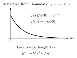
The boundary condition fixes the decay length $1/\kappa$ and the negative energy. The curve shows the wavefunction relative to its endpoint value; the dashed line is its tangent at the boundary. A Dirichlet endpoint excludes this state even though the differential expression in the interior is unchanged.

There is no contradiction with the expression being called a free kinetic energy. Integration by parts for the Robin realization gives

$$\langle\psi,H\psi\rangle =\frac{\hbar^2}{2m}\int_0^\infty|\psi'(x)|^2dx +\frac{\hbar^2\gamma}{2m}|\psi(0)|^2.$$

The boundary contribution can be negative. The endpoint represents additional physical information, for example an effective interaction at a boundary. The example shows why a domain is part of a Hamiltonian; the general theory is in Self-Adjoint Extensions.

A state can evolve without having a time derivative

A self-adjoint Hamiltonian defines a unitary group on the entire Hilbert space. Thus every state vector has a well-defined orbit $U(t)\psi$. The strong derivative at $t=0$, however, exists exactly for vectors in $D(H)$ and equals $-iH\psi/\hbar$.

The expression $i\hbar\dot\psi=H\psi$ therefore describes a stronger regularity statement than the existence of unitary evolution. A vector with a sufficiently heavy high-energy tail may lie outside $D(H)$ while still evolving normally. Stone’s Theorem makes the distinction precise. The point is to preserve the physically meaningful evolution rather than discard states because a convenient differential notation fails.

Spectral probabilities do not require normalizable eigenvectors

Position on the line has no nonzero $L^2$ eigenvector at a definite point. Nevertheless, it has a spectral measure, and the probability of a detector region $\Delta$ is

$$\langle\psi,E_X(\Delta)\psi\rangle =\int_\Delta|\psi(x)|^2dx.$$

This formula remains meaningful even though the probability of every singleton is zero for an ordinary wavepacket. Projection-Valued Measures supplies the general construction; Distribution Theory Minimum explains the generalized notation $|x\rangle$. Keeping the two roles separate prevents divergent normalization factors from being mistaken for probabilities.

A controlled approximation states what its error controls

Finite basis calculations, semiclassical expansions, and effective Hamiltonians are central to quantum mechanics. A rigorous treatment need not claim they are exact. It states the parameter regime, the error measure, and the conclusion that survives the approximation.

For instance, convergence of state vectors in norm controls probabilities of bounded effects. It does not automatically control an unbounded energy expectation. A strong operator limit need not be uniform over all possible input states. The convergence primer gives concrete examples. This is useful when deciding whether a numerical cutoff supports a statement about one wavepacket, an energy window, or an entire spectrum.

Exercise: verify the boundary energy

For the Robin bound state above, compute the derivative integral and boundary term separately. Check that their sum reproduces the eigenvalue.

Solution

$\int|\psi_\kappa'|^2dx=\kappa^2$ because the state is normalized. The endpoint term is $\gamma|\psi_\kappa(0)|^2=-2\kappa^2$. Their sum is $-\kappa^2$, giving $E=-\hbar^2\kappa^2/(2m)$. Dropping the boundary term would produce a positive number and a wrong physical prediction.

References

• Hall, Brian C., Quantum Theory for Mathematicians, Graduate Texts in Mathematics 267, Springer, 2013, doi:10.1007/978-1-4614-7116-5 — domains, spectral observables, and quantum evolution.
• Teschl, Gerald, Mathematical Methods in Quantum Mechanics: With Applications to Schrödinger Operators, 2nd ed., Graduate Studies in Mathematics 157, American Mathematical Society, 2014, author’s edition — self-adjoint boundary problems and spectral dynamics.