Schmidt Decomposition in Hilbert Space

Every normalizable vector in a bipartite Hilbert tensor product has a finite or countable Schmidt expansion. Infinite-dimensional factors do not replace the Schmidt sum by a continuum integral: the relevant operator is Hilbert–Schmidt and therefore compact. The canonical Schmidt Decomposition article supplies finite-matrix calculations and physical interpretation; this page proves the Hilbert-space extension and its approximation bounds.

Helpful background. Hilbert–Schmidt Operators and Compact Operators supply singular values. Algebraic Tensor Products and Completion supplies the completed state space.

A bipartite vector defines a compact operator

Let $\mathcal H_A,\mathcal H_B$ be separable complex Hilbert spaces. To keep the construction linear, use the conjugate Hilbert space $\overline{\mathcal H_B}$. Its vector $\bar y$ corresponds antilinearly to $y\in\mathcal H_B$.

For an algebraic tensor $\Psi=\sum_jx_j\otimes y_j$, define

$$T_\Psi:\overline{\mathcal H_B}\longrightarrow\mathcal H_A, \qquad T_\Psi\bar y=\sum_jx_j\langle y,y_j\rangle.$$

Our inner products are linear in the second argument, so the right side is antilinear in $y$ and linear in $\bar y$. This conjugation is essential; overlooking it causes the familiar transpose mistakes in coefficient formulas.

For an orthonormal basis $(f_k)$ of $\mathcal H_B$, Parseval gives

$$\|T_\Psi\|_2^2 =\sum_k\|T_\Psi\bar f_k\|^2 =\|\Psi\|^2.$$

Consequently the correspondence extends by completion to an isometry from $\mathcal H_A\otimes\mathcal H_B$ onto the Hilbert–Schmidt operators from $\overline{\mathcal H_B}$ to $\mathcal H_A$. Finite-rank maps supply a dense range. Every $T_\Psi$ is compact, even when both Hilbert spaces are infinite-dimensional.

The compact spectral theorem gives paired modes

Apply the compact positive spectral theorem to $T_\Psi^*T_\Psi$. For its nonzero eigenvalues choose orthonormal eigenvectors $\bar v_n$:

$$T_\Psi^*T_\Psi\bar v_n=s_n^2\bar v_n, \qquad s_n>0.$$

Set $u_n=s_n^{-1}T_\Psi\bar v_n$. The eigenvalue equation proves that the $u_n$ are orthonormal. The singular-value expansion converges in Hilbert–Schmidt norm, and the isometry above converts it into

$$\Psi=\sum_ns_nu_n\otimes v_n, \qquad \sum_ns_n^2=\|\Psi\|^2.$$

This is the Schmidt theorem. For a normalized vector the squared coefficients form a probability distribution. There are at most countably many nonzero coefficients, and an infinite list can accumulate only at zero.

The reduced states have nonzero eigenvalues $s_n^2$. More precisely, $\rho_A=T_\Psi T_\Psi^*$, while $T_\Psi^*T_\Psi$ represents the conjugate of $\rho_B$ on $\overline{\mathcal H_B}$. These identities follow by testing against bounded local operators and using the defining property of partial trace. The zero-eigenvalue complements need not have equal dimensions.

Finite Schmidt truncation has an exact error

Order the coefficients nonincreasingly and let

$$\Psi_r=\sum_{n=1}^rs_nu_n\otimes v_n, \qquad \delta_r=\sum_{n>r}s_n^2.$$

Orthogonality yields $\|\Psi-\Psi_r\|^2=\delta_r$. This is the smallest squared Hilbert-norm error achievable by any unnormalized vector of Schmidt rank at most $r$.

To prove optimality, translate a competing vector into a rank-at-most-$r$ Hilbert–Schmidt map $K$ and let $P$ project onto its range. Then

$$\|T_\Psi-K\|_2^2 \geq\|(I-P)T_\Psi\|_2^2 =\|T_\Psi\|_2^2-\operatorname{Tr}(PT_\Psi T_\Psi^*).$$

Writing the last trace in the $u_n$ eigenbasis shows it is at most $\sum_{n=1}^rs_n^2$: the weights $\langle u_n,Pu_n\rangle$ lie between zero and one and sum to at most $r$. The truncated singular-value expansion attains the bound.

For a normalized input and $\delta_r<1$, normalize the approximation as $\widehat\Psi_r=\Psi_r/\sqrt{1-\delta_r}$. Its overlap with the original vector is $\sqrt{1-\delta_r}$, so

$$\|\Psi-\widehat\Psi_r\|^2 =2\bigl(1-\sqrt{1-\delta_r}\bigr).$$

The pure-state trace-distance formula gives distance $\sqrt{\delta_r}$ between their density operators. Partial trace cannot increase this distance, so the same value bounds the error in either reduced state.

A geometric spectrum gives controlled cutoffs

For $0<q<1$, consider

$$\Psi_q=\sqrt{1-q}\sum_{n=0}^\infty q^{n/2}|n,n\rangle.$$

The terms are already paired orthonormal modes, and the geometric series proves normalization. Keeping $n=0,\ldots,r-1$ discards probability $\delta_r=q^r$. The normalized pure-state trace distance is therefore $q^{r/2}$.

The marginal distance is smaller in this example: it equals $\delta_r$. Both reduced states are diagonal in the same Schmidt basis. Renormalization increases the retained probabilities by a total of $\delta_r$, while deleting the tail removes the same total, giving trace distance $\tfrac12(\delta_r+\delta_r)=\delta_r$. The joint pure state also contains coherences between the retained and discarded modes, which explains its larger distance $\sqrt{\delta_r}$.

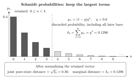
For $q=0.6$ and rank $r=4$, the light bars begin the infinite discarded tail. Its total probability is $0.1296$, while the normalized joint pure-state trace distance is $0.36$. The marginal trace distance is exactly the tail probability. Distances use $D(\rho,\sigma)=\tfrac12\|\rho-\sigma\|_1$.

To make the joint pure-state distance at most $\varepsilon\in(0,1)$, it suffices to choose $r\geq2\log(\varepsilon)/\log(q)$. Both logarithms are negative. As $q$ approaches one, the required rank grows, although every fixed $q<1$ still defines an ordinary Hilbert-space vector.

The formal endpoint with equal weights on infinitely many modes cannot be normalized. It is not a missing continuous version of the Schmidt theorem. Schmidt Decomposition Caveats separates this issue from generalized eigenvectors and mixed-state decompositions.

Exercises

1. If $s_n=C/n$ for $n\geq1$, give an upper bound on the trace distance after normalized rank-$r$ truncation.

Solution

The tail obeys $\delta_r=C^2\sum_{n>r}n^{-2}\leq C^2/r$. The pure-state trace distance is $\sqrt{\delta_r}\leq C/\sqrt r$. Infinite Schmidt rank does not prevent controlled approximation, but this polynomial tail is slower than the geometric example.

2. Can a nonzero Schmidt coefficient have infinite multiplicity in a normalizable vector?

Solution

No. If $s>0$ appeared infinitely often, the sum of squared coefficients would diverge. This is also the finite-multiplicity statement for nonzero eigenvalues of a compact operator. The zero eigenspace may have arbitrary dimension and contributes no terms to the expansion.

References

• Hall, Brian C., Quantum Theory for Mathematicians, Graduate Texts in Mathematics 267, Springer, 2013 — tensor products, compact operators, and Schmidt decomposition. Publisher.
• Holevo, Alexander S., Quantum Systems, Channels, Information: A Mathematical Introduction, second revised and expanded edition, De Gruyter, 2019 — bipartite normal states and reduced spectra. Publisher.
• Simon, Barry, Trace Ideals and Their Applications, second edition, Mathematical Surveys and Monographs 120, American Mathematical Society, 2005 — Hilbert–Schmidt singular values and finite-rank approximation. Publisher.