Holonomy

Holonomy is the transformation produced by parallel transport around a closed loop. If a connection transports data along a path, holonomy is what remains when the path returns to its starting point.

For a loop $C$ based at $p$,

$$U_C:E_p\to E_p.$$

In a one-dimensional phase fiber, $U_C$ is a phase. In a higher-dimensional vector bundle, it is a matrix acting on the fiber over $p$.

Helpful background. Parallel Transport explains the transport equation; Integration on Manifolds explains when Stokes’ theorem applies.

Closed loops and phase comparison

Transport along an open path compares different fibers. A closed path returns to the original fiber, so the final vector can be compared directly with the initial one. For a phase fiber this comparison is a complex number of unit modulus; for a larger fiber it is a matrix.

From Parallel Transport to Holonomy

Let $\gamma:[0,T]\to M$ be a path with $\gamma(0)=\gamma(T)=p$. Parallel transport along $\gamma$ defines a map

$$U_\gamma:E_p\to E_p.$$

Using the connection convention

$$\nabla=d+\Gamma,$$

the transport operator in a local frame is

$$U_\gamma = \operatorname{P}\exp \left( - \oint_\gamma \Gamma \right).$$

The symbol $\operatorname{P}$ denotes path ordering. It is needed when the connection matrices at different points do not commute.

For an open path, the transported object lives in a different fiber at the end. For a closed loop, the initial and final fibers are the same, so the transport map can be directly compared with the identity.

Abelian Phase Holonomy

For a U(1) phase connection, it is common to write

$$\Gamma=-iA,$$

where $A$ is a real one-form. In a frame periodic around the loop $C$, the holonomy is

$$U_C = \exp \left( i\oint_C A \right).$$

The phase

$$\gamma[C] = \oint_C A$$

is defined modulo $2\pi$ when only the phase factor $e^{i\gamma[C]}$ is observable.

Under an abelian gauge transformation

$$A\mapsto A-d\chi,$$

the closed-loop integral changes by

$$\oint_C A \mapsto \oint_C A-\oint_C d\chi.$$

If $\chi$ is single-valued around the loop, then

$$\oint_C d\chi=0.$$

More generally the gauge transformation $e^{i\chi}$ can be single-valued even when a continuous branch of $\chi$ changes by $2\pi k$ around the loop. Then $\oint d\chi=2\pi k$ and $e^{i\gamma[C]}$ is still unchanged. Gauge invariance concerns this phase factor, not a particular real-valued branch of $\gamma$.

Curvature Flux Formula

If $C=\partial\Sigma$ and a smooth gauge is available on the whole spanning surface $\Sigma$, Stokes theorem gives

$$\oint_C A = \int_\Sigma dA = \int_\Sigma F.$$

Therefore

$$U_C = \exp \left( i\int_\Sigma F \right).$$

This is the common “phase equals curvature flux” formula. The hypotheses are important:

• $C$ must bound the chosen oriented surface $\Sigma$;
• the connection must be smooth on that surface;
• the same gauge or compatible patching data must be valid;
• singularities or removed points inside the loop must be treated explicitly.

When those hypotheses fail, the holonomy may still be well defined, but it cannot be computed by a naive single-patch Stokes calculation.

Flat Connections Can Have Holonomy

Curvature is local. Holonomy can also detect global topology.

On a circle with angular coordinate $\theta$, consider

$$A=\alpha\,d\theta.$$

The curvature vanishes:

$$F=dA=0,$$

but the holonomy around the circle is

$$U_{S^1} = \exp \left( i\int_0^{2\pi}\alpha\,d\theta \right) = e^{i2\pi\alpha}.$$

Thus a flat connection need not have trivial holonomy on a space with noncontractible loops. Homotopy and Winding explains the loop classes behind this statement. This is the basic mathematical pattern behind Aharonov–Bohm-type phases.

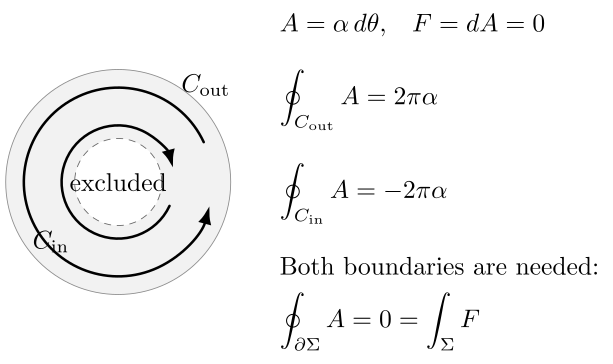
The accessible annulus has zero curvature, but its outer boundary alone can have a nonzero phase integral. Stokes’ theorem includes both boundary components, whose integrals cancel. A disk spanning only the outer loop would cross the excluded region.

Berry Phase as Holonomy

For a nondegenerate eigenstate over parameter space, the Berry connection is locally

$$A_n = i\langle n(R)\rvert d n(R)\rangle.$$

In a smooth frame periodic around the closed loop $C$, the Berry holonomy is

$$e^{i\gamma_n[C]} = \exp \left( i\oint_C A_n \right).$$

If $C=\partial\Sigma$ and a smooth eigenstate gauge exists on $\Sigma$, then

$$\gamma_n[C] = \int_\Sigma F_n \quad \operatorname{mod} 2\pi, \qquad F_n=dA_n.$$

For the $+1$ eigenline of $\hat{\mathbf n}\cdot\boldsymbol\sigma$, with $A=i\langle n|dn\rangle$, a loop of directions on the unit sphere gives

$$\gamma = -\frac{\Omega}{2} \quad \operatorname{mod} 2\pi,$$

where $\Omega$ is the oriented solid angle enclosed by the loop. The physical derivation and sign conventions are discussed in Berry Phase. The opposite eigenline gives the opposite sign.

When the curvature is integrated over a closed two-dimensional parameter space rather than a spanning surface for one loop, the quantized invariant is a Chern number.

Aharonov–Bohm Phase as Holonomy

In the Aharonov–Bohm effect, a charged particle travels in a region where the magnetic field can vanish along the accessible paths, while the vector potential has nontrivial circulation around an excluded flux region.

With minimal coupling convention $p\mapsto p-qA$, the phase factor around a closed loop is

$$\exp \left( \frac{iq}{\hbar} \oint_C A_i\,dx^i \right).$$

If the loop encloses magnetic flux $\Phi$, then

$$\oint_C A_i\,dx^i = \Phi,$$

so the Aharonov–Bohm phase is

$$\Delta\varphi = \frac{q\Phi}{\hbar}$$

in this unit convention. Some electromagnetic unit systems insert a factor of $c$ in the denominator; the invariant content is that the phase is the charge times gauge-potential holonomy in units of $\hbar$.

The crucial geometric point is that local field strength on the accessible path is not the whole story. The loop winds around a region removed from the configuration space, and the connection can have nontrivial holonomy around that missing region.

Nonabelian Holonomy

For a higher-dimensional fiber, the holonomy is a matrix:

$$U_C = \operatorname{P}\exp \left( - \oint_C\Gamma \right).$$

Under a change of frame at the base point, $U_C$ changes by conjugation:

$$U_C\mapsto g(p)^{-1}U_Cg(p).$$

The matrix itself depends on the chosen frame, but conjugacy-invariant information does not. Examples include eigenvalues and traces such as

$$\operatorname{Tr}U_C.$$

In physics, trace-like loop observables are often called Wilson loops. Detailed Wilson-loop calculations in band topology and gauge theory belong to later specialized pages; the mathematical idea is already present here.

Holonomy Group

Fix a base point $p$. The holonomies of all loops based at $p$ form a group under composition:

$$\operatorname{Hol}_p(\nabla) = \{U_C:C\text{ is a loop based at }p\}.$$

Transport around the trivial loop gives the identity. Reversing a loop gives the inverse. Concatenating loops gives multiplication.

The holonomy group is a compact way to summarize the possible loop transports of a connection. Infinitesimal loops probe curvature; large loops also probe topology and global patching.

Local Curvature versus Global Holonomy

The relationship between curvature and holonomy has two layers:

• infinitesimal holonomy around very small loops is governed by curvature;
• global holonomy around large or noncontractible loops may contain topological winding information not visible from local curvature on a single patch.

This is why the statements

$$F=0$$

and

$$U_C=I\quad\text{for every closed loop }C$$

are not equivalent on every space. For a smooth flat connection over a connected, simply connected region, parallel transport is path independent and every loop has trivial holonomy. On a punctured plane, circle, torus, or bundle with nontrivial patching, flat connections can still have nontrivial loop phases.

Common Mistakes

• Treating holonomy as a property of a point rather than a loop and a connection.
• Assuming that zero curvature on the path implies zero holonomy around the path.
• Applying Stokes theorem across a surface where the gauge is singular or the physical region is removed.
• Forgetting that abelian holonomy is a phase modulo $2\pi$.
• Treating nonabelian holonomy matrices as gauge invariant rather than conjugacy covariant.
• Confusing Berry holonomy in parameter space with ordinary motion in physical space.
• Mixing electromagnetic unit conventions in the Aharonov–Bohm phase.

Exercises

1. Show that $\oint_C A$ is unchanged by $A\mapsto A-d\chi$ when $\chi$ is single-valued around $C$.

Solution

The transformed integral is

$$\oint_C(A-d\chi) = \oint_C A-\oint_C d\chi.$$

Since $d\chi$ is an exact differential,

$$\oint_C d\chi = \chi(\text{end})-\chi(\text{start}).$$

For a closed loop and a single-valued $\chi$, the start and end values agree, so

$$\oint_C d\chi=0.$$

2. Let $F=F_0\,dx\wedge dy$ on a rectangle of area $ab$. What is the abelian holonomy phase if $C$ is the positively oriented boundary and a smooth $A$ satisfies $dA=F$?

Solution

By Stokes theorem,

$$\oint_C A = \int_\Sigma F = F_0ab.$$

Therefore

$$U_C = \exp(iF_0ab).$$

3. For $A=\alpha\,d\theta$ on a circle, compute the holonomy around one counterclockwise loop.

Solution

The integral is

$$\oint_{S^1}A = \int_0^{2\pi}\alpha\,d\theta = 2\pi\alpha.$$

Thus

$$U_{S^1}=e^{i2\pi\alpha}.$$

Although $dA=0$, the loop can have nontrivial holonomy because the circle is not simply connected.

4. If a nonabelian holonomy transforms as $U_C\mapsto g^{-1}U_Cg$, show that $\operatorname{Tr}U_C$ is invariant.

Solution

Using cyclicity of trace,

$$\operatorname{Tr}(g^{-1}U_Cg) = \operatorname{Tr}(gg^{-1}U_C) = \operatorname{Tr}U_C.$$

Thus the trace is independent of the frame at the base point.

5. A charged particle encircles magnetic flux $\Phi$ once. In the convention used above, what is the Aharonov–Bohm phase?

Solution

The phase is

$$\Delta\varphi = \frac{q}{\hbar} \oint_C A_i\,dx^i.$$

Since the loop encloses flux $\Phi$,

$$\oint_C A_i\,dx^i=\Phi.$$

Therefore

$$\Delta\varphi = \frac{q\Phi}{\hbar}.$$

6. A spin-$1/2$ Berry loop encloses oriented solid angle $\Omega$. What is the usual phase factor for the aligned state when $\gamma=-\Omega/2$?

Solution

The Berry phase is

$$\gamma=-\frac{\Omega}{2} \quad \operatorname{mod}2\pi.$$

The corresponding phase factor is

$$e^{i\gamma} = \exp \left( -\frac{i\Omega}{2} \right).$$

References

• M. V. Berry, “Quantal phase factors accompanying adiabatic changes”, Proceedings of the Royal Society A 392, 45-57, 1984.
• M. Nakahara, Geometry, Topology and Physics, 2nd ed., CRC Press, 2003.
• B. Simon, “Holonomy, the quantum adiabatic theorem, and Berry’s phase”, Physical Review Letters 51, 2167-2170, 1983.