Convolution

Convolution combines two functions by sliding one against the other and integrating the overlap. In Fourier analysis, it is important because convolution in one representation becomes multiplication in the transformed representation.

For functions on the real line, a common convention is

$$(f*g)(x) = \int_{-\infty}^{\infty} f(x-y)g(y)\,dy.$$

The operation is associative and commutative under standard hypotheses, but in applications the order often carries interpretation: a source is acted on by a response kernel, or a wavefunction is mixed by a potential.

Convolution as a Sum of Shifted Responses

Convolution appears whenever a linear translation-invariant system builds its output by superposing shifted copies of one fixed response:

$$u(x) = \int_{-\infty}^{\infty} G(x-y)f(y)\,dy = (G*f)(x).$$

Here $f$ is a source and $G$ is the response to a point source. This is the full-line, translation-invariant version of a Green-function formula. When boundaries or nonuniform coefficients break translation invariance, the kernel usually depends on both variables separately as $G(x,\xi)$ instead of only on $x-\xi$.

Convolution Theorem in the k Convention

For the ordinary $k$-space convention

$$F(k) = \int_{-\infty}^{\infty} f(x)e^{-ikx}\,dx, \qquad f(x) = \frac{1}{2\pi} \int_{-\infty}^{\infty} F(k)e^{ikx}\,dk,$$

the convolution theorem is

$$\mathcal F_k[f*g](k) = F(k)G(k).$$

The product theorem is the companion identity:

$$\mathcal F_k[fg](k) = \frac{1}{2\pi} (F*G)(k).$$

The placement of the factor $1/(2\pi)$ depends on the Fourier convention. This is one reason to check Fourier Transform Conventions before comparing formulas across sources.

Proof of the Convolution Theorem

For $f,g\in L^1(\mathbb R)$, the double integral is absolutely integrable, so Fubini’s theorem permits the interchange:

$$\begin{aligned} \mathcal F_k[f*g](k) &= \int_{-\infty}^{\infty} e^{-ikx} \int_{-\infty}^{\infty} f(x-y)g(y)\,dy\,dx \\ &= \int_{-\infty}^{\infty} g(y)e^{-iky}\,dy \int_{-\infty}^{\infty} f(z)e^{-ikz}\,dz \\ &= G(k)F(k). \end{aligned}$$

The second line uses $z=x-y$. For distributions and less regular functions, this calculation must be interpreted with the appropriate functional-analytic hypotheses.

The Unitary Momentum Convention

The wave-mechanics pages use the unitary $p$ convention

$$\widetilde f(p) = \frac{1}{\sqrt{2\pi\hbar}} \int_{-\infty}^{\infty} e^{-ipx/\hbar}f(x)\,dx.$$

With this symmetric normalization,

$$\mathcal F_p[f*g](p) = \sqrt{2\pi\hbar}\, \widetilde f(p)\widetilde g(p).$$

The product theorem becomes

$$\mathcal F_p[fg](p) = \frac{1}{\sqrt{2\pi\hbar}} \int_{-\infty}^{\infty} \widetilde f(q)\widetilde g(p-q)\,dq.$$

Thus a local product in position space becomes momentum mixing. In one-dimensional quantum mechanics, if $V(x)$ multiplies a wavefunction $\psi(x)$, then in momentum space the potential term has the form

$$\mathcal F_p[V\psi](p) = \frac{1}{\sqrt{2\pi\hbar}} \int_{-\infty}^{\infty} \widetilde V(q)\phi(p-q)\,dq,$$

where $\phi$ is the momentum-space wavefunction. Local potentials are therefore not usually diagonal in momentum representation.

For the operator dictionary that uses this fact, see Position and Momentum Representations.

Delta Functions and Shifts

The delta distribution is the identity for convolution:

$$(\delta*f)(x) = f(x).$$

More generally, let

$$\delta_a(x) = \delta(x-a).$$

Then

$$(\delta_a*f)(x) = f(x-a).$$

This identity says that a shifted point source produces a shifted response. It is the simplest way to remember why a Green function $G(x-a)$ is the response to a source located at $a$ in a translation-invariant problem.

Green Functions as Convolution Kernels

Let $L$ be a translation-invariant differential operator on the real line. If

$$LG=\delta,$$

then the solution of

$$Lu=f$$

is formally

$$u=G*f.$$

Fourier transformation turns the differential equation into algebra. If $L$ has Fourier symbol $\ell(k)$, then

$$\ell(k)U(k)=F(k), \qquad U(k)=\frac{F(k)}{\ell(k)}.$$

The Green function is the inverse transform of $1/\ell(k)$, and multiplication by $1/\ell(k)$ in Fourier space is convolution by $G$ in position space.

For example, with

$$L = -\frac{d^2}{dx^2}+\kappa^2, \qquad \kappa>0,$$

the Fourier symbol is

$$\ell(k)=k^2+\kappa^2.$$

Thus

$$G(x) = \int_{-\infty}^{\infty} \frac{dk}{2\pi} \frac{e^{ikx}}{k^2+\kappa^2} = \frac{e^{-\kappa\lvert x\rvert}}{2\kappa}.$$

Then

$$u(x) = \int_{-\infty}^{\infty} \frac{e^{-\kappa\lvert x-y\rvert}}{2\kappa} f(y)\,dy$$

solves

$$\left( -\frac{d^2}{dx^2}+\kappa^2 \right)u(x) = f(x)$$

under the full-line decay condition. For the broader operator-and-boundary-condition perspective, see Green Functions.

Worked Example: Two Rectangular Pulses

Let $f(x)=g(x)=1$ for $0\le x\le a$, with $a>0$, and zero otherwise. In the convolution integral, $g(y)$ requires $y\in[0,a]$, while $f(x-y)$ requires $y\in[x-a,x]$. The integrand equals one on the overlap of these intervals, so the answer is the overlap length:

$$(f*g)(x)= \begin{cases} x,&0\le x\le a,\\ 2a-x,&a\le x\le2a,\\ 0,&\text{otherwise}. \end{cases}$$

Two rectangles therefore convolve into a triangle. The result peaks at $x=a$, when the intervals overlap completely, and has area $a^2=(\int f)(\int g)$. Notice that convolution reverses and shifts one input before measuring overlap; a cross-correlation uses a different reversal/conjugation convention.

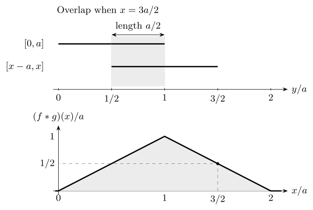
For two unit-height rectangles on $[0,a]$, convolution equals the length shared by $[0,a]$ and $[x-a,x]$. At $x=3a/2$, that length is $a/2$. The lower plot shows the entire answer, with both axes scaled by $a$.

Response Interpretation

In response language, $G$ is an impulse response. A general source $f(y)$ is decomposed into point sources, each point source produces a shifted response $G(x-y)$, and integration adds all responses:

$$u(x) = \int G(x-y)f(y)\,dy.$$

Fourier space says the same thing differently:

$$U(k) = G(k)F(k).$$

The response kernel becomes a transfer function. Frequencies or momenta for which $G(k)$ is large are amplified; those for which $G(k)$ is small are suppressed. In quantum scattering, propagators and resolvents play the same structural role, though their boundary prescriptions and normalization conventions must be stated explicitly.

Common Mistakes

• Confusing convolution with pointwise multiplication.
• Dropping the factor of $2\pi$ or $\sqrt{2\pi\hbar}$ when changing Fourier conventions.
• Using a translation-invariant convolution formula when the boundary conditions require a two-variable Green function $G(x,\xi)$.
• Treating products or convolutions of distributions as automatically defined.
• Confusing convolution with correlation, where one of the functions is reversed or conjugated.
• Forgetting that a local potential in position space generally becomes a momentum-space convolution.

Related Topics

• Fourier Transform
• Inverse Fourier Transform
• Plancherel and Parseval Theorems
• Delta Function
• Fourier Transform Table
• Position and Momentum Representations

Exercises

1. Prove the convolution theorem in the $k$ convention.

Solution

Start from the definition:

$$\mathcal F_k[f*g](k) = \int e^{-ikx} \int f(x-y)g(y)\,dy\,dx.$$

Set $z=x-y$, so $x=z+y$ and $dx=dz$. Then

$$\mathcal F_k[f*g](k) = \int g(y)e^{-iky}\,dy \int f(z)e^{-ikz}\,dz = G(k)F(k).$$

Because multiplication is commutative, this is $F(k)G(k)$.

2. Let $\delta_a(x)=\delta(x-a)$. Compute $(\delta_a*f)(x)$.

Solution

Using the convolution definition,

$$(\delta_a*f)(x) = \int \delta_a(x-y)f(y)\,dy = \int \delta(x-y-a)f(y)\,dy.$$

The delta distribution evaluates the integrand at $y=x-a$, giving

$$(\delta_a*f)(x) = f(x-a).$$

3. In the unitary $p$ convention, why does a product $V(x)\psi(x)$ become a convolution in momentum space?

Solution

Write both factors by inverse Fourier transforms:

$$V(x) = \frac{1}{\sqrt{2\pi\hbar}} \int \widetilde V(q)e^{iqx/\hbar}\,dq,$$

and

$$\psi(x) = \frac{1}{\sqrt{2\pi\hbar}} \int \phi(r)e^{irx/\hbar}\,dr.$$

Multiplying and transforming back gives a delta constraint $q+r=p$, so

$$\mathcal F_p[V\psi](p) = \frac{1}{\sqrt{2\pi\hbar}} \int \widetilde V(q)\phi(p-q)\,dq.$$

Thus each output momentum $p$ receives contributions from many input momenta.

4. Let $G$ satisfy $LG=\delta$ for a translation-invariant operator $L$. Show formally that $u=G*f$ solves $Lu=f$.

Solution

Because $L$ acts on the $x$ variable and is translation-invariant,

$$L(G*f) = (LG)*f.$$

Using $LG=\delta$ gives

$$L(G*f) = \delta*f = f.$$

This formal argument assumes the convolution is defined and that $L$ can be moved through the integral. Boundary-value problems require the corresponding Green-function kernel and domain conditions.

References

• G. B. Arfken, H. J. Weber, and F. E. Harris, Mathematical Methods for Physicists, 7th ed., Academic Press, 2013.
• E. N. Economou, Green’s Functions in Quantum Physics, 3rd ed., Springer, 2006.
• G. B. Folland, Fourier Analysis and Its Applications, American Mathematical Society, 2009.
• G. F. Roach, Green’s Functions, 2nd ed., Cambridge University Press, 1982.
• E. M. Stein and R. Shakarchi, Fourier Analysis: An Introduction, Princeton University Press, 2003.