Completeness and Orthonormal Bases

A complete orthonormal basis is an orthonormal family large enough to approximate every Hilbert-space vector in norm. It is the infinite-dimensional version of the finite-dimensional statement

$$I = \sum_i \lvert e_i\rangle\langle e_i\rvert,$$

but the infinite-dimensional word “complete” carries convergence content that must not be suppressed.

The finite-dimensional algebra is Orthonormal Bases. This page explains what changes in Hilbert spaces such as $L^2(\mathbb R)$.

For why standard quantum Hilbert spaces usually admit countable complete orthonormal bases, see Separable Hilbert Spaces.

Helpful background. Review finite orthonormal bases to compute expansion coefficients and projection errors.

Orthonormal Systems

Let $\mathcal H$ be a Hilbert space. A sequence or countable family

$$\{e_1,e_2,\ldots\}$$

is orthonormal if

$$\langle e_m\vert e_n\rangle = \delta_{mn}.$$

For any finite linear combination

$$f = \sum_{n=1}^{N} c_n e_n,$$

orthonormality gives

$$\lVert f\rVert^2 = \sum_{n=1}^{N}\lvert c_n\rvert^2.$$

This part is exactly like finite-dimensional linear algebra.

Completeness

The orthonormal family is complete if its closed linear span is the whole Hilbert space:

$$\overline{\operatorname{span}\{e_n:n\ge1\}} = \mathcal H.$$

Equivalently, the only vector orthogonal to every $e_n$ is the zero vector:

$$\langle e_n\vert\psi\rangle=0 \quad \text{for all }n \quad \Longrightarrow \quad \psi=0.$$

The closure is essential. Infinite sums usually converge as limits of partial sums, not as finite combinations.

Expansion Coefficients

If $\{e_n\}$ is complete and orthonormal, then every $\psi\in\mathcal H$ has coefficients

$$c_n = \langle e_n\vert\psi\rangle.$$

The expansion is

$$\psi = \sum_{n=1}^{\infty} c_n e_n,$$

meaning

$$\lim_{N\to\infty} \left\lVert \psi - \sum_{n=1}^{N}c_n e_n \right\rVert = 0.$$

This is convergence in Hilbert-space norm. It does not automatically mean pointwise convergence of representative functions.

Parseval and Inner Products

For a complete orthonormal basis, Parseval’s identity says

$$\lVert\psi\rVert^2 = \sum_{n=1}^{\infty} \lvert c_n\rvert^2, \qquad c_n=\langle e_n\vert\psi\rangle.$$

If

$$\phi = \sum_n d_n e_n, \qquad \psi = \sum_n c_n e_n,$$

then

$$\langle\phi\vert\psi\rangle = \sum_n d_n^*c_n.$$

This is the infinite-dimensional analogue of taking dot products of coordinate columns.

Partial-Sum Projectors

Define

$$P_N = \sum_{n=1}^{N} \lvert e_n\rangle\langle e_n\rvert.$$

Then $P_N\psi$ is the best approximation to $\psi$ inside the finite-dimensional subspace spanned by $e_1,\ldots,e_N$:

$$P_N\psi = \sum_{n=1}^{N} \langle e_n\vert\psi\rangle e_n.$$

Completeness means

$$P_N\psi\to\psi$$

for every $\psi\in\mathcal H$, with convergence in norm. This is sometimes called strong convergence of $P_N$ to the identity. It is weaker than saying the operators converge in operator norm.

Norm Convergence Versus Pointwise Convergence

For $L^2$ spaces, norm convergence means

$$\int \lvert f_N(x)-f(x)\rvert^2\,dx \to0.$$

It does not say that $f_N(x)\to f(x)$ at every point. Nor does it say that the series can be differentiated term by term.

This distinction matters in quantum mechanics because probabilities depend on integrals of squared moduli. A basis expansion can converge perfectly well as a state expansion even when the pointwise behavior of the representative functions is delicate.

Fourier Example

On an interval of length $L$, the functions

$$e_n(x) = \frac{1}{\sqrt L} e^{2\pi i n x/L}, \qquad n\in\mathbb Z,$$

form a complete orthonormal basis of $L^2([0,L])$. No endpoint values are required of a general $L^2$ vector. Periodic boundary conditions become relevant when these functions are used as eigenfunctions of a particular differential operator.

For $f\in L^2([0,L])$,

$$f(x) \sim \sum_{n\in\mathbb Z} c_n e_n(x), \qquad c_n = \int_0^L e_n(x)^*f(x)\,dx.$$

The symbol $\sim$ is a useful reminder: the expansion converges to $f$ in $L^2$ norm. Extra hypotheses are needed for stronger pointwise statements. The finite-interval expansion is developed in Periodic Functions and Fourier Series, while full-line transform conventions are collected in Fourier Transform.

Bound-State Example

For the infinite square well on $0\lt x\lt L$, the normalized eigenfunctions

$$u_n(x) = \sqrt{\frac{2}{L}} \sin\frac{n\pi x}{L}, \qquad n=1,2,\ldots,$$

form a complete orthonormal system in all of $L^2(0,L)$. The Dirichlet boundary conditions characterize the Hamiltonian domain, not the entire state space: a general square-integrable function need not even have well-defined endpoint values.

A normalizable state in the well can be expanded as

$$\psi(x) = \sum_{n=1}^{\infty} c_n u_n(x), \qquad c_n = \int_0^L u_n(x)^*\psi(x)\,dx,$$

with convergence in $L^2$ norm. The physical model is Infinite Square Well, and the mathematical background is Sturm–Liouville Theory.

Example: expanding a constant in sine functions

Take $\psi(x)=1/\sqrt L$ on $(0,L)$. Direct integration gives

$$c_n=\frac{\sqrt2}{n\pi}\bigl[1-(-1)^n\bigr].$$

Equivalently,

$$c_n=\begin{cases}2\sqrt2/(n\pi),&n\text{ odd},\\0,&n\text{ even}. \end{cases}$$

Thus a constant has a sine expansion even though every partial sum vanishes at the endpoints. Endpoint values have measure zero and do not obstruct $L^2$ convergence. The approximation error is exactly

$$\left\|\psi-\sum_{n=1}^N c_nu_n\right\|_2^2 =1-\frac{8}{\pi^2}\sum_{\substack{n\le N\\n\text{ odd}}}\frac1{n^2}.$$

The same state is outside the Dirichlet Hamiltonian’s form domain: its energy sum is proportional to $\sum_n n^2|c_n|^2$, which diverges. Being a state and having finite mean energy are different requirements.

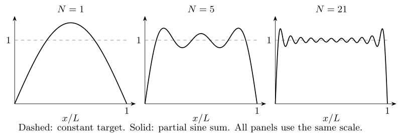
Sine expansion of the constant function, with $x$ measured in units of $L$ and amplitude in units of $1/\sqrt L$. Endpoint values remain zero in every finite sum, while the squared error integrated over the interval decreases. The narrowing endpoint regions do not prevent $L^2$ convergence.

Discrete Bases Versus Generalized Bases

A countable complete orthonormal basis consists of Hilbert-space vectors. Position kets $\lvert x\rangle$ and momentum kets $\lvert p\rangle$ are not normalizable Hilbert-space vectors, so they are not orthonormal bases in this strict sense.

Physicists still write formal resolution relations such as

$$I = \int \lvert x\rangle\langle x\rvert\,dx,$$

but these belong to the language of generalized eigenvectors and distributions. The practical position-momentum representation is introduced in Position and Momentum Representations.

Common Mistakes

• Treating “complete” as a decorative word rather than a statement about closed spans.
• Assuming norm convergence implies pointwise convergence.
• Differentiating or multiplying an infinite expansion without checking convergence and domains.
• Confusing a countable orthonormal basis with a continuum of generalized eigenvectors.
• Forgetting boundary conditions when choosing basis functions for a differential Hamiltonian.
• Assuming that a set of mutually orthogonal functions is complete without proof or a theorem.
• Treating a truncated expansion as exact without estimating the discarded norm.

References

• G. B. Folland, Fourier Analysis and Its Applications, American Mathematical Society, 2009.
• B. C. Hall, Quantum Theory for Mathematicians, Springer, 2013.
• M. Reed and B. Simon, Methods of Modern Mathematical Physics, Volume I: Functional Analysis, Academic Press, 1980.
• R. Shankar, Principles of Quantum Mechanics, 2nd ed., Springer, 1994.

Exercises

1. Let $\{e_n\}$ be a complete orthonormal basis and let $c_n=\langle e_n\vert\psi\rangle$. What does

$$\psi = \sum_{n=1}^{\infty}c_n e_n$$

mean?

Solution

It means convergence in Hilbert-space norm:

$$\lim_{N\to\infty} \left\lVert \psi - \sum_{n=1}^{N}c_n e_n \right\rVert = 0.$$

It does not automatically assert pointwise convergence of functions.

2. Suppose $\{e_n\}$ is complete orthonormal and $\langle e_n\vert\psi\rangle=0$ for every $n$. What is $\psi$?

Solution

Completeness implies that the only vector orthogonal to every basis vector is the zero vector. Therefore $\psi=0$.

3. If $\psi=\sum_n c_n e_n$ in a complete orthonormal basis and $\lVert\psi\rVert=1$, what does Parseval’s identity give?

Solution

Parseval’s identity gives

$$1 = \lVert\psi\rVert^2 = \sum_n \lvert c_n\rvert^2.$$

In quantum mechanics, these squared moduli become probabilities when the basis corresponds to a projective measurement context.

4. Why are position kets not a countable orthonormal basis of $L^2(\mathbb R)$?

Solution

The objects $\lvert x\rangle$ are generalized eigenvectors, not normalizable Hilbert-space vectors. They are labeled by a continuum and satisfy delta-normalization formally. A countable orthonormal basis of a Hilbert space consists of actual Hilbert-space vectors with finite norm.