Why Postulates Matter

A postulate package specifies how a physical theory turns preparations, transformations, composite systems, and measurements into quantitative predictions. It identifies the theory’s primitive objects and the rules that connect them.

Postulates are not ceremonial preliminaries. Without them, symbols such as $\lvert\psi\rangle$, $\rho$, $A$, and $H$ have no agreed physical role. Yet a postulate list is not a complete model of an experiment, a derivation from data alone, or an answer to every interpretive question.

This page explains the job and logical status of postulates. The compact list is Minimal Postulates; the remaining pages translate that package into finite-dimensional, wave-mechanical, and density-operator forms.

Helpful background. Quantum states and the Born rule introduce the objects whose logical roles are compared here.

What Counts as a Postulate

A postulate is a rule adopted as part of a theory’s starting structure. Within that package it is not proved from earlier rules. It constrains what mathematical objects represent physical situations and how those objects generate predictions.

Several neighboring kinds of statement should not be conflated with postulates:

• A theorem follows logically from the postulates plus stated mathematical assumptions.
• A model assumption selects a particular system, Hamiltonian, state preparation, detector, boundary condition, or approximation.
• A convention fixes notation or coordinates without changing predictions.
• An empirical regularity summarizes observed behavior that motivates, tests, or constrains the theory.
• An interpretive claim assigns ontology or explanatory meaning beyond the shared predictive rules.

For example, assigning the Hilbert space $\mathbb C^2$ to an ideal spin-$1/2$ degree of freedom uses the state-space framework but also models the relevant system as two dimensional. Choosing

$$H = \frac{\hbar\omega}{2}\sigma_z$$

is a model assumption, not a universal postulate of quantum mechanics. Choosing whether $\sigma_z$ is diagonal with the $+1$ entry first is a convention. Deriving the transition probability under that $H$ is a calculation.

The boundary between “postulate” and “theorem” depends on the chosen primitives. A rule stated independently in one presentation may be derived inside a broader framework in another. Logical role is package relative.

A Compact Theory Specification

A laboratory prediction involves four layers:

1. physical procedures and modeling assumptions;
2. mathematical representatives;
3. a probability rule;
4. comparison with experimental data.

In a modern finite-dimensional notation, a single trial may be summarized by

$$\begin{aligned} \text{preparation }P &\longmapsto \rho_P, \\ \text{transformation }T &\longmapsto \mathcal T, \\ \text{measurement }M &\longmapsto \{E_a\}_a, \\ & \sum_a E_a=I. \end{aligned}$$

Here $\rho_P$ is positive with trace one, each $E_a$ is positive, and $\mathcal T$ is a linear, completely positive, trace-preserving transformation. The predicted outcome probabilities are

$$p(a\mid P,T,M) = \operatorname{Tr} \left[ \mathcal T(\rho_P)E_a \right].$$

For a closed system, $\mathcal T(\rho)=U\rho U^\dagger$. For a pure state and projective measurement,

$$\rho_P = \lvert\psi\rangle\langle\psi\rvert, \qquad E_a=P_a,$$

and the trace rule becomes

$$p(a) = \langle\psi\rvert U^\dagger P_a U \lvert\psi\rangle.$$

The postulates specify which assignments and transformations are allowed and how this probability is computed. The physical model specifies which $\rho_P$, $U$, and $P_a$ describe the apparatus at hand.

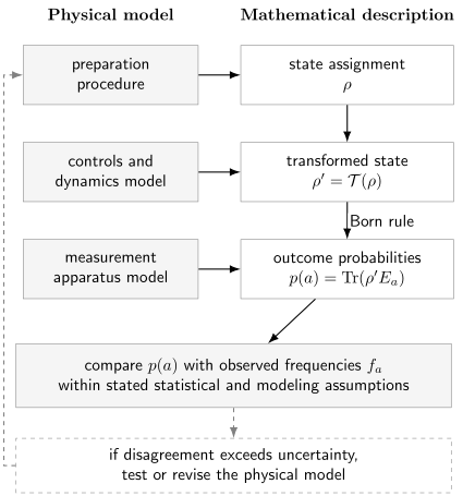
Postulates organize the formal arrows and probability rule. Experimental agreement tests the entire physical modeling package, including preparation, dynamics, measurement, and statistical assumptions.

Different Equivalent Packages

There is no single sacred textbook list. Common packages include:

• an abstract Hilbert-space presentation using rays, self-adjoint operators, the Born rule, unitary evolution, and tensor products;
• a wave-mechanics presentation using $\psi(x)$, differential operators, normalization, and the Schrödinger equation;
• a density-operator presentation using positive trace-one operators, measurement effects, channels, and partial traces;
• a finite-dimensional quantum-information presentation using matrices, qubits, instruments, and tensor-product registers.

These packages are equivalent only when a translation preserves the relevant operational predictions within a stated domain. For a pure state,

$$\lvert\psi\rangle \longleftrightarrow \rho_\psi = \lvert\psi\rangle\langle\psi\rvert$$

preserves every probability:

$$\langle\psi\rvert E_a\lvert\psi\rangle = \operatorname{Tr}(\rho_\psi E_a).$$

Likewise,

$$\psi(x) = \langle x\vert\psi\rangle$$

is the position representation of an abstract state vector, not a new physical theory.

Apparent equivalence can fail when domains, boundary conditions, superselection sectors, or infinite-dimensional operator issues are suppressed. Equivalent Formulations gives the canonical comparison.

Textbook Postulates and Reconstruction Programs

Textbook postulates usually begin with the mature Hilbert-space formalism and state how to use it. A reconstruction asks whether that mathematical formalism can be derived from more operational or information-theoretic principles.

Examples of reconstruction programs use assumptions about distinguishability, composition, reversible transformations, purification, causality, or information capacity. They clarify which structural features separate quantum theory from nearby probabilistic theories.

These programs do not produce one universally accepted unique derivation. Different reconstructions:

• choose different primitive operational notions;
• address finite-dimensional or other restricted domains;
• assume different continuity, composition, or causality conditions;
• optimize for different explanatory goals.

Their value is diagnostic: they expose which physical principles do work in deriving the familiar formalism. They do not make empirical input unnecessary, because the reconstruction principles themselves must be motivated, interpreted, and tested.

For examples with explicitly different starting assumptions, see Hardy (2001), Chiribella, D’Ariano, and Perinotti (2011), and Masanes and Müller (2011) in the references. Compare their scope as well as their conclusion.

Postulates and Interpretations

The shared predictive postulates do not by themselves decide what the quantum state ultimately represents, whether a state update is ontic or epistemic, or why an individual run yields one definite recorded outcome.

For an ideal projective measurement,

$$p(a) = \operatorname{Tr}(\rho P_a)$$

predicts the outcome distribution. A selective update rule then predicts conditional probabilities for later measurements. Those rules are sufficient for repeatability checks and sequential-measurement calculations.

They do not uniquely answer:

• whether the state is a physical field, information, a relation, or part of another ontology;
• whether all branches persist;
• whether collapse is fundamental, effective, or inferential;
• why this particular outcome occurred in one trial.

Interpretations may add claims about these questions while retaining the same ordinary laboratory probabilities. Such additions should be labeled as interpretive rather than smuggled into the shared formalism. See What the Postulates Do Not Say.

What Postulates Cannot Do Alone

A postulate package does not supply the physical model for a particular problem. It does not determine:

• the Hamiltonian of an atom or molecule;
• masses, charges, coupling constants, or external fields;
• a wavefunction’s boundary conditions;
• which detector observable or POVM models an apparatus;
• which degrees of freedom may be neglected;
• the accuracy of an approximation;
• the preparation history or experimental noise model.

For example, the Schrödinger equation specifies how a chosen Hamiltonian generates evolution:

$$i\hbar \frac{d}{dt} \lvert\psi(t)\rangle = H(t)\lvert\psi(t)\rangle.$$

It does not tell us whether $H$ should describe a Coulomb potential, harmonic trap, spin coupling, lattice model, or effective open-system interaction. That information comes from physics beyond the abstract postulate.

Experiment tests predictions made by the postulates and all these modeling choices. A discrepancy does not identify which ingredient failed without further analysis.

Worked Example: One Prediction in Two Packages

Prepare a two-level system in

$$\lvert+x\rangle = \frac{ \lvert0\rangle+\lvert1\rangle }{ \sqrt2 }$$

and measure in the basis $\{\lvert0\rangle,\lvert1\rangle\}$. The state-vector package uses

$$P_0=\lvert0\rangle\langle0\rvert$$

and predicts

$$\begin{aligned} p(0) &= \langle+x\rvert P_0 \lvert+x\rangle \\ &= \frac12. \end{aligned}$$

The density-operator package represents the preparation by

$$\rho = \lvert+x\rangle\langle+x\rvert = \frac12 \begin{pmatrix} 1&1\\ 1&1 \end{pmatrix}.$$

Its prediction is

$$\begin{aligned} p(0) &= \operatorname{Tr}(\rho P_0) \\ &= \frac12. \end{aligned}$$

The symbols differ, but the state and measurement translations preserve the probability. This is operational equivalence in a simple pure-state setting.

Worked Example: Composition Adds New States

Suppose $A$ and $B$ are qubits. The composition rule assigns

$$\mathcal H_{AB} = \mathcal H_A\otimes\mathcal H_B, \qquad \dim\mathcal H_{AB}=4.$$

Product preparations give vectors such as

$$\lvert0\rangle_A\lvert1\rangle_B.$$

The tensor-product space also contains

$$\lvert\Phi^+\rangle_{AB} = \frac{ \lvert00\rangle+\lvert11\rangle }{ \sqrt2 },$$

which cannot be written as $\lvert\alpha\rangle_A\lvert\beta\rangle_B$. Entanglement is not appended by a separate empirical formula after composition; it follows from the state-space structure assigned to composites.

The local states are

$$\rho_A=\rho_B=\frac I2,$$

even though the joint state is pure. The example shows why a compact structural rule can have far-reaching consequences and why changing a composition postulate changes the theory’s possible correlations.

Exercises

1. Classify each statement as a postulate-level rule, theorem, model assumption, or convention:

• pure states are represented by rays;
• $H=(\hbar\omega/2)\sigma_z$ for a particular spin apparatus;
• unitary evolution preserves inner products;
• the ordered basis is $\{\lvert0\rangle,\lvert1\rangle\}$ rather than $\{\lvert1\rangle,\lvert0\rangle\}$.

Solution

Within the standard package, representing pure states by rays is a postulate-level rule. Choosing the specific Hamiltonian is a model assumption. Preservation of inner products is a theorem following from unitarity:

$$\langle U\phi\vert U\psi\rangle = \langle\phi\rvert U^\dagger U \lvert\psi\rangle = \langle\phi\vert\psi\rangle.$$

The ordering of the basis is a convention. Changing it consistently changes matrix positions but not predictions.

2. A source prepares $\lvert+z\rangle$, a spin evolves under a known Hamiltonian $H$, and an apparatus measures $S_x$. Identify the preparation, transformation, measurement, and probability rule.

Solution

The preparation is represented by

$$\rho_P = \lvert+z\rangle\langle+z\rvert.$$

For a closed interval of duration $t$, the transformation is

$$\mathcal T(\rho) = U(t)\rho U^\dagger(t), \qquad U(t)=e^{-iHt/\hbar}$$

when $H$ is time independent. The $S_x$ measurement has projectors

$$P_\pm = \lvert\pm x\rangle\langle\pm x\rvert.$$

The outcome probabilities are

$$p(\pm) = \operatorname{Tr} \left[ U(t)\rho_P U^\dagger(t)P_\pm \right].$$

3. Explain why a global phase is representational redundancy while a relative phase can affect predictions.

Solution

Replacing $\lvert\psi\rangle$ by $e^{i\alpha}\lvert\psi\rangle$ leaves the density operator unchanged:

$$e^{i\alpha} \lvert\psi\rangle\langle\psi\rvert e^{-i\alpha} = \lvert\psi\rangle\langle\psi\rvert.$$

Every Born-rule probability is therefore unchanged. A relative phase in

$$\frac{ \lvert0\rangle+e^{i\phi}\lvert1\rangle }{ \sqrt2 }$$

changes off-diagonal density-matrix elements and can change measurements in a basis that recombines $\lvert0\rangle$ and $\lvert1\rangle$.

4. Prove that the ket and density-operator packages give the same probability for a pure state and measurement effect $E_a$.

Solution

Set $\rho_\psi=\lvert\psi\rangle\langle\psi\rvert$. Then cyclicity of the trace gives

$$\begin{aligned} \operatorname{Tr}(\rho_\psi E_a) &= \operatorname{Tr} \bigl( \lvert\psi\rangle\langle\psi\rvert E_a \bigr) \\ &= \langle\psi\rvert E_a \lvert\psi\rangle. \end{aligned}$$

Thus the translation preserves every single-outcome probability. For full equivalence one must also translate transformations, composites, and conditional operations.

5. Which structural rule makes entangled states possible? Show that the Bell state cannot be a product.

Solution

The composition rule assigns the tensor product

$$\mathcal H_{AB} = \mathcal H_A\otimes\mathcal H_B.$$

Suppose

$$\frac{ \lvert00\rangle+\lvert11\rangle }{ \sqrt2 } = \bigl( a\lvert0\rangle_A+b\lvert1\rangle_A \bigr) {}\otimes \bigl( c\lvert0\rangle_B+d\lvert1\rangle_B \bigr).$$

Matching coefficients would require

$$\begin{aligned} ac&=\frac1{\sqrt2}, & ad&=0, \\ bc&=0, & bd&=\frac1{\sqrt2}. \end{aligned}$$

The nonzero first and last equations require $a,b,c,d\ne0$, contradicting $ad=bc=0$. Therefore the state is not a product.

6. Why is choosing the Coulomb Hamiltonian for hydrogen not itself a universal quantum postulate?

Solution

The postulate-level dynamics rule says how a self-adjoint Hamiltonian generates evolution. The Coulomb Hamiltonian identifies masses, charges, coordinates, and an interaction appropriate to one physical model:

$$H = \frac{\boldsymbol p^2}{2\mu} - \frac{e^2}{4\pi\epsilon_0 r}.$$

Its form comes from modeling the hydrogen atom and the electromagnetic interaction, together with approximations such as nonrelativistic motion and a suitable treatment of the nucleus. Other systems use different Hamiltonians without changing the general quantum postulates.

7. Give one measurement question answered by the standard postulates and one not answered by them alone.

Solution

Given a state and a measurement, the postulates answer the probability of each outcome and, with an instrument or update rule, the conditional probabilities for later measurements.

They do not by themselves decide the ultimate ontology of the state, whether a selective update is a physical collapse or an information update, or why one individual trial yields one particular outcome. Those are interpretive or foundational questions beyond the shared probability algorithm.

8. Two authors give postulate lists of different lengths. What must be checked before concluding that they describe different theories?

Solution

One must compare primitives, scope, and predictions. A rule stated independently in one list may be derived from a broader primitive in the other. For example, a separate projective update rule may be included inside a general instrument formalism.

Construct translation maps between states, transformations, measurements, and composites, then check whether

$$p(a\mid P,T,M)$$

is preserved for every procedure in the shared domain. Also compare background assumptions such as dimension, continuity, superselection, and allowed measurements. Different numbering or length alone does not imply different physics.

References

• G. Chiribella, G. M. D’Ariano, and P. Perinotti, “Informational derivation of quantum theory,” Physical Review A 84, 012311 (2011). DOI: 10.1103/PhysRevA.84.012311.
• P. A. M. Dirac, The Principles of Quantum Mechanics, 4th edition, Oxford University Press, 1958.
• L. Hardy, “Quantum theory from five reasonable axioms” (2001). arXiv:quant-ph/0101012.
• L. Masanes and M. P. Müller, “A derivation of quantum theory from physical requirements,” New Journal of Physics 13, 063001 (2011). DOI: 10.1088/1367-2630/13/6/063001.
• M. A. Nielsen and I. L. Chuang, Quantum Computation and Quantum Information, 10th anniversary edition, Cambridge University Press, 2010. Cambridge DOI.
• A. Peres, Quantum Theory: Concepts and Methods, Kluwer Academic Publishers, 1995. Springer DOI.
• J. J. Sakurai and J. Napolitano, Modern Quantum Mechanics, 3rd edition, Cambridge University Press, 2020.
• J. von Neumann, Mathematical Foundations of Quantum Mechanics, English translation, Princeton University Press, 1955.