Crank–Nicolson Method

Crank–Nicolson advances Schrödinger evolution through a linear solve. For a fixed Hermitian Hamiltonian, its update is a Cayley transform: it preserves norm exactly in exact arithmetic and is second-order accurate in time. Stability permits a large step without exponential growth; it does not make that step physically accurate.

Helpful background. The numerical Schrödinger equation defines the represented initial-value problem.

Deriving the Cayley update

Apply the trapezoidal rule to $i\hbar\dot\psi=H\psi$ with fixed $H$:

$$i\hbar\frac{\psi_{n+1}-\psi_n}{h} =H\frac{\psi_{n+1}+\psi_n}{2}.$$

Rearranging gives

$$\left(I+\frac{ihH}{2\hbar}\right)\psi_{n+1} =\left(I-\frac{ihH}{2\hbar}\right)\psi_n.$$

Let $a=h/(2\hbar)$. The update is $U_{\rm CN}=(I+iaH)^{-1}(I-iaH)$. Since the two factors are commuting functions of Hermitian $H$, $U_{\rm CN}^\dagger U_{\rm CN}=I$. It also commutes with $H$, so the discrete energy expectation is conserved for a fixed Hamiltonian.

Do not form the inverse. Factor the left matrix once when $h$ and $H$ are fixed, then reuse the factorization. A one-dimensional nearest-neighbor spatial stencil gives a tridiagonal solve; more general sparse matrices may incur fill-in.

Phase accuracy on one eigenmode

For $H|E\rangle=E|E\rangle$, the update multiplier is

$$u(E)=\frac{1-ihE/(2\hbar)}{1+ihE/(2\hbar)} =e^{-2i\arctan[hE/(2\hbar)]}.$$

Its magnitude is one, but its phase differs from $-hE/\hbar$. Expanding,

$$\frac{2}{h}\arctan\frac{hE}{2\hbar} =\frac{E}{\hbar} -\frac{h^2E^3}{12\hbar^3}+O(h^4).$$

Thus phase error accumulates over long times. Large-energy modes can have badly distorted frequencies even though the trajectory remains bounded.

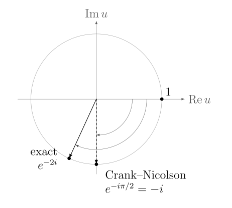
One eigenmode step with $hE/\hbar=2$, starting from multiplier $1$. The exact phase is $-2$ radians; Crank–Nicolson gives $-\pi/2$. Both points have modulus one, so a normalization check misses the angular error.

A scalar energy shift changes the numerical phase error of this rational approximation; account for its global phase and test the relevant energy bandwidth.

Nonorthogonal and time-dependent cases

In a fixed nonorthogonal basis with overlap $S>0$, use

$$\left(S+\frac{ihH}{2\hbar}\right)c_{n+1} =\left(S-\frac{ihH}{2\hbar}\right)c_n.$$

This preserves $c^\dagger Sc$ in exact arithmetic. Euclidean norm is not the physical norm unless the basis is orthonormal.

For time-dependent $H$, a midpoint-frozen Hermitian matrix used in both factors gives a second-order implicit-midpoint step that remains unitary. The literal endpoint trapezoidal formula, with $H(t_n)$ on the right and $H(t_{n+1})$ on the left, is also second order under smoothness assumptions but is not generally exactly unitary. State which version is implemented.

Non-Hermitian absorbers intentionally violate norm conservation. Interpret norm loss through the absorber model rather than applying the closed-system proof.

Solver residuals and refinement

An inexact linear solve adds its own error. Record the residual of the linear system, vary its tolerance below the time-step error, and check norm drift over the full trajectory. Solving each step to a loose tolerance can accumulate a systematic error even when the method’s exact update is unitary.

For a two-level diagonal Hamiltonian and an equal superposition, compare the computed relative phase after a fixed total time with the exact one. Halving $h$ should reduce the leading phase error by roughly four. Also run a forward/backward check; reversibility alone cannot detect the method’s modified eigenfrequencies.

Exercises

For $hE/\hbar=2$, compare the exact one-step phase magnitude with that of Crank–Nicolson.

Solution

The exact phase magnitude is $2$ radians. Crank–Nicolson gives $2\arctan(1)=\pi/2\approx1.5708$ radians. Both multipliers have unit modulus, but the phase error is about $0.4292$ radians in a single step.

References

• Crank, J., and P. Nicolson, “A practical method for numerical evaluation of solutions of partial differential equations of the heat-conduction type,” Proceedings of the Cambridge Philosophical Society 43, 50–67 (1947); 1996 reprint — the implicit second-order scheme.
• Hairer, E., C. Lubich, and G. Wanner, Geometric Numerical Integration, 2nd ed., Springer, 2006 — midpoint integration, invariants, and modified dynamics.