Local and Global Observables

A local observable asks a question about one subsystem. A correlation observable compares paired results, and a general joint measurement can distinguish states that share every local statistic. These distinctions concern both which probabilities are measured and how the apparatus changes the state.

A statement such as “measure observable $A$ on subsystem $A$” is shorthand for an operator on the whole composite Hilbert space. If

$$\mathcal H_{AB} = \mathcal H_A\otimes\mathcal H_B,$$

then an observable $M_A$ available to the first subsystem is represented globally as

$$M_A\otimes I_B.$$

The identity factor is not decorative. It records which degrees of freedom the operation leaves untouched, makes dimensions and operator products well-defined, and distinguishes a local observable from a correlation observable such as $A\otimes B$.

Helpful background. Operators on Composite Systems explains identity factors; Reduced Density Operators explains which information a local state contains.

Local operators

Use bounded operators below, including all finite matrices; unbounded observables need domain and moment conditions as in the operator discussion. Let $X_A$ act on $\mathcal H_A$. Its natural embedding into the composite operator algebra is

$$\iota_A(X_A) = X_A\otimes I_B.$$

On a product vector,

$$(X_A\otimes I_B) \left( \lvert\psi\rangle_A\otimes\lvert\phi\rangle_B \right) = \left( X_A\lvert\psi\rangle_A \right) \otimes \lvert\phi\rangle_B.$$

The action extends by linearity and continuity to every vector in $\mathcal H_A\otimes\mathcal H_B$, including entangled vectors. Similarly, an operator local to $B$ is embedded as

$$\iota_B(Y_B) = I_A\otimes Y_B.$$

The embedding preserves the operator algebra:

$$\begin{aligned} \iota_A(X_A Y_A) &= \iota_A(X_A)\iota_A(Y_A), \\ \iota_A(X_A^\dagger) &= \iota_A(X_A)^\dagger, \\ \iota_A(I_A) &= I_A\otimes I_B. \end{aligned}$$

Consequently, Hermitian operators remain Hermitian, projectors remain projectors, and unitary operators remain unitary after embedding.

Spectra and degeneracy

Suppose

$$M_A = \sum_a m_a P_a$$

is the spectral decomposition of a finite-dimensional observable. Then

$$M_A\otimes I_B = \sum_a m_a \left( P_a\otimes I_B \right).$$

The numerical eigenvalues are unchanged, but their multiplicities grow. If the eigenspace of $m_a$ in $\mathcal H_A$ has dimension $g_a$, then its eigenspace in the composite system has dimension

$$g_a\,\dim\mathcal H_B.$$

This extra degeneracy reflects that the local observable does not distinguish any states of subsystem $B$.

Operators on distinct factors commute

For bounded operators $X_A$ and $Y_B$,

$$\begin{aligned} (X_A\otimes I_B)(I_A\otimes Y_B) &= X_A\otimes Y_B \\ &\qquad= (I_A\otimes Y_B)(X_A\otimes I_B). \end{aligned}$$

Therefore

$$\left[ X_A\otimes I_B,\, I_A\otimes Y_B \right] =0.$$

This compatibility is an algebraic fact about tensor factors. It does not, by itself, establish relativistic locality: a tensor-factor label need not represent a spacetime region, and relativistic theories impose additional causal structure.

Product observables

If $A$ and $B$ are Hermitian, then

$$A\otimes B$$

is a Hermitian observable on the composite system. It acts on both factors:

$$(A\otimes B) \left( \lvert\psi\rangle_A\otimes\lvert\phi\rangle_B \right) = \left( A\lvert\psi\rangle_A \right) \otimes \left( B\lvert\phi\rangle_B \right).$$

If $A\lvert a\rangle=a\lvert a\rangle$ and $B\lvert b\rangle=b\lvert b\rangle$, then

$$(A\otimes B) \lvert a\rangle\lvert b\rangle = ab\, \lvert a\rangle\lvert b\rangle.$$

Thus the eigenvalues of a product observable are products of local eigenvalues.

A product observable is not the same thing as a local observable. It usually probes a joint correlation. When $A$ and $B$ are measured locally on the two subsystems, multiplying the two outcomes estimates $\langle A\otimes B\rangle$.

Factorization in product states

For a product density operator

$$\rho_{AB} = \rho_A\otimes\rho_B,$$

the expectation value factorizes:

$$\begin{aligned} \langle A\otimes B\rangle &= \operatorname{Tr}_{AB} \left[ (\rho_A\otimes\rho_B)(A\otimes B) \right] \\ &= \operatorname{Tr}_A(\rho_A A)\, \operatorname{Tr}_B(\rho_B B). \end{aligned}$$

For a general joint state, define the connected correlation

$$\operatorname{Cov}_{\rho}(A,B) = \langle A\otimes B\rangle_\rho - \langle A\otimes I_B\rangle_\rho \langle I_A\otimes B\rangle_\rho.$$

Every product state has zero connected correlation for every pair $A,B$. The converse requires factorization for a sufficiently complete family of operators; one vanishing covariance does not prove that the state is a product state.

Beyond a single product

Most composite observables are not one tensor product. In finite dimensions, any operator can be expanded as a sum

$$O_{AB} = \sum_{\mu,\nu} c_{\mu\nu}\, F_\mu^{(A)}\otimes G_\nu^{(B)}$$

using operator bases on the two subsystems. Whether such an observable is operationally local, a correlation measurement, or a genuinely joint measurement depends on the complete operator and on how it is implemented, not merely on the fact that it can be written as a sum of tensor products.

The finite product-operator expansion is derived in Operators on Composite Systems.

Sums, interactions, and locality

For noninteracting subsystems, a Hamiltonian often has the form

$$H_0 = H_A\otimes I_B + I_A\otimes H_B.$$

The first term changes only $A$ and the second changes only $B$. An interaction adds a term such as

$$H_{\mathrm{couple}} = J\,Z_A\otimes Z_B.$$

Although this interaction is a single product operator, it is not local to either subsystem. It couples them and can generate correlations or entanglement.

Locality can also depend on the dynamical picture. An operator that is local at the reference time may spread under interacting Heisenberg evolution:

$$M_A(t) = U^\dagger(t) \left( M_A\otimes I_B \right) U(t).$$

When $U(t)$ is generated by an interaction, $M_A(t)$ generally cannot be written as $M_A'(t)\otimes I_B$. This is operator spreading, not a contradiction of the original tensor-factor definition.

Expectation values from reduced states

Let

$$\rho_A = \operatorname{Tr}_B\rho_{AB}.$$

The defining property of the partial trace is

$$\operatorname{Tr}_{AB} \left[ \rho_{AB}(M_A\otimes I_B) \right] = \operatorname{Tr}_A(\rho_A M_A).$$

Every expectation value accessible through an observable local to $A$ can therefore be computed from $\rho_A$ alone. Conversely, in finite dimensions, these expectation values for all Hermitian $M_A$ determine $\rho_A$ uniquely. This is the operational content of a reduced state.

The reduced state does not determine

$$\langle A\otimes B\rangle,$$

because that quantity depends on correlations retained in $\rho_{AB}$. Nor does $\rho_A$ generally determine which global preparation produced it. Many different pure and mixed joint states can share the same marginal.

For a product state,

$$\rho_{AB}=\rho_A\otimes\rho_B,$$

the two reduced states contain enough information to reconstruct the joint state. For correlated states they do not.

Local measurements

Projective measurements

Let $\{P_a\}$ be a projective measurement on $A$:

$$P_aP_{a'} = \delta_{aa'}P_a, \qquad \sum_a P_a=I_A.$$

On the composite Hilbert space, the measurement projectors are

$$P_a\otimes I_B.$$

For a joint state $\rho_{AB}$, the Born probability is

$$\begin{aligned} p(a) &= \operatorname{Tr}_{AB} \left[ \rho_{AB}(P_a\otimes I_B) \right] \\ &= \operatorname{Tr}_A(\rho_A P_a). \end{aligned}$$

For a device implementing the Lüders instrument and a selected outcome with $p(a)>0$, the joint state is

$$\rho_{AB|a} = \frac{ (P_a\otimes I_B) \rho_{AB} (P_a\otimes I_B) }{p(a)}.$$

The first equation concerns outcome statistics; the second concerns post-measurement state assignment. Keeping those roles separate prevents a large class of measurement mistakes. See Projective Measurement for the distinction between outcome projectors and their implementation.

General measurement effects

For a local POVM on $A$, let

$$E_a\ge0, \qquad \sum_a E_a=I_A.$$

The corresponding joint-system effects are $E_a\otimes I_B$, and

$$\begin{aligned} p(a) &= \operatorname{Tr}_{AB} \left[ \rho_{AB}(E_a\otimes I_B) \right] \\ &= \operatorname{Tr}_A(\rho_A E_a). \end{aligned}$$

The effects determine probabilities but do not, by themselves, specify the conditional output state of the measured subsystem or the joint system. That requires a measurement instrument. The conditional state of an untouched partner is an exception: it is fixed by the effect and the initial joint state, as shown in Conditional States. The distinction is developed in Generalized Measurements Overview.

Measurements on both subsystems

If $\{E_a\}$ is a POVM on $A$ and $\{F_b\}$ is a POVM on $B$, their product measurement has joint effects

$$E_a\otimes F_b$$

and probabilities

$$p(a,b) = \operatorname{Tr}_{AB} \left[ \rho_{AB}(E_a\otimes F_b) \right].$$

Summing over $b$ gives

$$\begin{aligned} p_A(a) &= \sum_b p(a,b) \\ &= \operatorname{Tr}_{AB} \left[ \rho_{AB} \left( E_a\otimes\sum_b F_b \right) \right] \\ &= \operatorname{Tr}_A(\rho_A E_a). \end{aligned}$$

The joint distribution can depend strongly on both measurement choices, while its local marginal depends only on the reduced state.

Two-qubit examples

A local spin observable

For two spin-$1/2$ systems, the $z$ component of the first spin is

$$S_z^{(A)} = \frac{\hbar}{2} \sigma_z\otimes I_2.$$

Its eigenvalues are $+\hbar/2$ and $-\hbar/2$. Each is twice degenerate because the second spin may independently be up or down.

For example,

$$S_z^{(A)} \lvert\uparrow\downarrow\rangle = \frac{\hbar}{2} \lvert\uparrow\downarrow\rangle,$$

whereas

$$S_z^{(A)} \lvert\downarrow\uparrow\rangle = -\frac{\hbar}{2} \lvert\downarrow\uparrow\rangle.$$

Local randomness and joint order

For

$$\lvert\Phi^+\rangle = \frac{ \lvert00\rangle+\lvert11\rangle }{\sqrt2},$$

each reduced state is $I_2/2$. Consequently,

$$\langle Z\otimes I\rangle=0, \qquad \langle I\otimes Z\rangle=0.$$

Yet the correlation observables satisfy

$$\langle Z\otimes Z\rangle=1, \qquad \langle X\otimes X\rangle=1.$$

Each local result is unbiased, but the paired results are perfectly correlated in either of these bases.

Now compare the separable mixed state

$$\rho_{\mathrm{cc}} = \frac12 \lvert00\rangle\langle00\rvert + \frac12 \lvert11\rangle\langle11\rvert.$$

It has the same reduced states and the same $Z\otimes Z$ correlation:

$$\langle Z\otimes Z\rangle_{\mathrm{cc}}=1.$$

However,

$$\langle X\otimes X\rangle_{\mathrm{cc}}=0.$$

No experiment confined to one subsystem distinguishes these two global states. A suitable joint correlation measurement does.

Ignoring and selecting remote outcomes

A trace-preserving local operation on B cannot change the reduced state of A. If its Kraus operators satisfy $\sum_\mu K_\mu^\dagger K_\mu=I_B$, then

$$\operatorname{Tr}_B\!\left[ \sum_\mu (I_A\otimes K_\mu)\rho_{AB}(I_A\otimes K_\mu^\dagger) \right]=\rho_A.$$

The proof moves only B-local factors through the partial trace and uses completeness; Local Measurement Statistics supplies the full argument. It applies to ignored outcomes, without conditioning on a selected record.

Knowing a remote result $b$ instead gives a conditional state $\rho_{A|b}$, defined only for $p(b)>0$. These states can differ, while

$$\sum_{b:p(b)>0}p(b)\rho_{A|b}=\rho_A.$$

The weighted average explains no-signaling: an observer who lacks the remote record sees the unchanged marginal distribution. Conditional States works through the selected subensembles.

Global Observables That Are Not Local

A global observable is any Hermitian operator on $\mathcal H_{AB}$. Some global observables are sums or products of local terms. Others are tied to entangled bases and cannot be reproduced by separately measuring $A$ and $B$ in fixed local bases.

The Bell-basis projectors are the standard two-qubit example:

$$\Pi_{\Phi^+} = \lvert\Phi^+\rangle\langle\Phi^+\rvert, \qquad \Pi_{\Phi^-} = \lvert\Phi^-\rangle\langle\Phi^-\rvert,$$

with analogous projectors for $\lvert\Psi^+\rangle$ and $\lvert\Psi^-\rangle$. A Bell-basis measurement distinguishes coherent superpositions of product-basis states. Measuring both qubits separately in the computational basis does not reveal the relative phase that distinguishes $\lvert\Phi^+\rangle$ from $\lvert\Phi^-\rangle$.

Global observables also appear in angular momentum. For two spins, the total spin operator

$$\mathbf S^2 = (\mathbf S_1+\mathbf S_2)^2$$

distinguishes singlet and triplet sectors. It is not the same information as separately measuring $S_{1z}$ and $S_{2z}$.

Measuring a product versus preserving its eigenspaces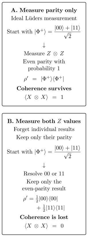

The same parity probabilities can accompany different state changes. Procedure A resolves only the even and odd subspaces; procedure B first resolves each $Z$ outcome. Both begin with the same Bell state. Forgetting a recorded distinction does not restore the coherence it removed.

Measuring Z locally on each qubit and reporting only the product of the two results reproduces the probabilities of $Z\otimes Z$. Its state change can differ from an ideal parity measurement.

The even and odd parity projectors are

$$P_+=|00\rangle\langle00|+|11\rangle\langle11|, \qquad P_-=|01\rangle\langle01|+|10\rangle\langle10|.$$

For the input $|\Phi^+\rangle$, both procedures report even parity with certainty. A Lüders parity measurement leaves this vector unchanged, because $P_+|\Phi^+\rangle=|\Phi^+\rangle$. Separate Z measurements followed by discarding their detailed records give

$$\rho_{\mathrm{out}} =\tfrac12|00\rangle\langle00|+\tfrac12|11\rangle\langle11|.$$

The coherence is lost even if the apparatus later reports only parity. A subsequent X-correlation measurement distinguishes the outputs: $\langle X\otimes X\rangle$ is respectively 1 and 0. Thus reproducing the distribution of an observable is weaker than reproducing its Lüders instrument.

Spin-Singlet Correlations

The spin singlet is

$$\lvert\Psi^-\rangle = \frac{ \lvert\uparrow\rangle_A\lvert\downarrow\rangle_B - \lvert\downarrow\rangle_A\lvert\uparrow\rangle_B }{\sqrt2}.$$

For any common axis $\hat n$,

$$\langle (\boldsymbol\sigma\cdot\hat n) \otimes (\boldsymbol\sigma\cdot\hat n) \rangle = -1.$$

Each local spin component has zero expectation:

$$\langle (\boldsymbol\sigma\cdot\hat n) \otimes I \rangle = 0, \qquad \langle I\otimes (\boldsymbol\sigma\cdot\hat n) \rangle = 0.$$

The singlet therefore separates three ideas: local observables, joint correlation observables, and rotationally invariant global structure.

Common pitfalls

One correlation cannot classify the state. A Bell state and a separable mixture can both have $\langle Z\otimes Z\rangle=1$. Their other correlations differ, as the X measurements above show.

Matching output labels does not match state changes. Grouping fine outcomes reproduces coarse probabilities but may destroy coherence within a coarse eigenspace.

Tensor-factor locality is not automatically spacetime locality. Different factors may describe spin and position of one particle. Relativistic causal claims need more structure than a vanishing tensor-factor commutator.

References

• P. Busch, P. Lahti, J.-P. Pellonpää, and K. Ylinen, Quantum Measurement, Springer, 2016.
• M. A. Nielsen and I. L. Chuang, Quantum Computation and Quantum Information, 10th anniversary ed., Cambridge University Press, 2010, chapter 2.
• J. Preskill, Lecture Notes for Physics 229: Quantum Information and Computation, chapter 2. Author notes.
• J. Watrous, The Theory of Quantum Information, Cambridge University Press, 2018, chapters 1–2. Author manuscript.

Exercises

1. Prove that bounded local operators on distinct factors commute:

$$\left[ X_A\otimes I_B,\, I_A\otimes Y_B \right] =0.$$

Solution

Use the tensor-product multiplication rule:

$$(X_A\otimes I_B)(I_A\otimes Y_B) = X_A\otimes Y_B,$$

and

$$(I_A\otimes Y_B)(X_A\otimes I_B) = X_A\otimes Y_B.$$

The two products are equal, so their difference vanishes.

2. Let $M_A$ have an eigenvalue $m$ with degeneracy $g$, and let $\dim\mathcal H_B=d_B$. Find the degeneracy of $m$ for $M_A\otimes I_B$.

Solution

Choose a basis $\{\lvert m,\alpha\rangle_A\}_{\alpha=1}^{g}$ for the eigenspace and any basis $\{\lvert j\rangle_B\}_{j=1}^{d_B}$ for $\mathcal H_B$. Then

$$(M_A\otimes I_B) \lvert m,\alpha\rangle_A\lvert j\rangle_B = m\, \lvert m,\alpha\rangle_A\lvert j\rangle_B.$$

There are $g d_B$ independent vectors of this form, so the composite degeneracy is $g d_B$.

3. For $\rho_{AB}=\rho_A\otimes\rho_B$, prove that every product-observable expectation factorizes.

Solution

Using multiplication and trace factorization,

$$\begin{aligned} \langle A\otimes B\rangle &= \operatorname{Tr}_{AB} \left[ (\rho_A A)\otimes(\rho_B B) \right] \\ &= \operatorname{Tr}_A(\rho_A A)\, \operatorname{Tr}_B(\rho_B B). \end{aligned}$$

Thus every connected correlation vanishes in a product state.

4. For the Bell state $\lvert\Phi^+\rangle$, calculate $\langle Z\otimes I\rangle$ and $\langle Z\otimes Z\rangle$ directly.

Solution

The local operator gives

$$(Z\otimes I)\lvert\Phi^+\rangle = \frac{ \lvert00\rangle-\lvert11\rangle }{\sqrt2},$$

which is orthogonal to $\lvert\Phi^+\rangle$. Therefore

$$\langle Z\otimes I\rangle=0.$$

By contrast, both $\lvert00\rangle$ and $\lvert11\rangle$ have eigenvalue $+1$ under $Z\otimes Z$, so

$$(Z\otimes Z)\lvert\Phi^+\rangle = \lvert\Phi^+\rangle,$$

and $\langle Z\otimes Z\rangle=1$.

5. Show that the Bell state and

$$\rho_{\mathrm{cc}} = \frac12\lvert00\rangle\langle00\rvert + \frac12\lvert11\rangle\langle11\rvert$$

have the same local $Z$ statistics and the same $\langle Z\otimes Z\rangle$, but different $\langle X\otimes X\rangle$.

Solution

Both reduced states are $I_2/2$, so either local $Z$ outcome is equally likely. In both global states, computational-basis outcomes agree, giving

$$\langle Z\otimes Z\rangle=1.$$

For the Bell state,

$$(X\otimes X)\lvert\Phi^+\rangle = \lvert\Phi^+\rangle,$$

so its $X\otimes X$ expectation is $1$. For either projector in $\rho_{\mathrm{cc}}$, $X\otimes X$ maps the basis vector to the other orthogonal basis vector. Hence each diagonal expectation vanishes and

$$\langle X\otimes X\rangle_{\mathrm{cc}}=0.$$

6. Let

$$\lvert\Psi_p\rangle = \sqrt p\,\lvert00\rangle + \sqrt{1-p}\,\lvert11\rangle.$$

For $0\le p\le1$, compute $\langle Z\otimes I\rangle$, $\langle X\otimes I\rangle$, and $\langle Z\otimes Z\rangle$.

Solution

The reduced state is

$$\rho_A = p\lvert0\rangle\langle0\rvert + (1-p)\lvert1\rangle\langle1\rvert.$$

Therefore

$$\langle Z\otimes I\rangle = \operatorname{Tr}(\rho_A Z) = 2p-1,$$

and

$$\langle X\otimes I\rangle = \operatorname{Tr}(\rho_A X) =0.$$

Both terms of the joint state have equal $Z$ outcomes, so

$$\langle Z\otimes Z\rangle=1.$$

7. Let a trace-preserving operation on $B$ have Kraus operators $\{K_\mu\}$. Prove that it leaves $\rho_A$ unchanged when its outcomes are ignored.

Solution

For any $M_A$, cyclicity of the full trace gives

$$\operatorname{Tr}_{AB} \left[ \rho'_{AB}(M_A\otimes I_B) \right] = \sum_\mu \operatorname{Tr}_{AB} \left[ \rho_{AB} \left( M_A\otimes K_\mu^\dagger K_\mu \right) \right].$$

Trace preservation implies

$$\sum_\mu K_\mu^\dagger K_\mu=I_B,$$

so the expression equals the original local expectation

$$\operatorname{Tr}_{AB} \left[ \rho_{AB}(M_A\otimes I_B) \right].$$

Since the equality holds for every $M_A$, the operators representing the two local states are equal:

$$\rho'_A=\rho_A.$$

8. Subsystem $B$ of $\lvert\Phi^+\rangle$ is measured in the computational basis. Find the conditional states of $A$ and verify that their unconditioned average is unchanged.

Solution

The two outcomes occur with probabilities

$$p(0)=p(1)=\frac12.$$

Conditioned on outcome $0$ at $B$, subsystem $A$ is assigned $\lvert0\rangle\langle0\rvert$. Conditioned on outcome $1$, it is assigned $\lvert1\rangle\langle1\rvert$. Averaging without access to the outcome gives

$$\begin{aligned} \sum_b p(b)\rho_{A|b} &= \frac12\lvert0\rangle\langle0\rvert + \frac12\lvert1\rangle\langle1\rvert \\ &= \frac{I_2}{2} = \rho_A. \end{aligned}$$

The remote result changes the conditional state, but ignoring that result leaves the local reduced state and all local statistics unchanged.

9. Bell-basis versus product-basis measurement. Why does measuring both qubits in the computational basis fail to distinguish $\lvert\Phi^+\rangle$ from $\lvert\Phi^-\rangle$?

Solution

The two states are

$$\lvert\Phi^\pm\rangle = \frac{ \lvert00\rangle\pm\lvert11\rangle }{\sqrt2}.$$

Computational-basis measurement gives probability $1/2$ for $00$ and $1/2$ for $11$ in both cases. The relative sign is phase information between the two branches, and it is not recorded by local computational-basis outcome probabilities.