EPR State Preview

An EPR state is an idealized continuous-variable entangled state with perfect correlation in one collective variable and perfect correlation in a compatible momentum variable. The original Einstein–Podolsky–Rosen example used two particles with a sharply defined relative position and total momentum.

Finite-width wavepackets and finite squeezing approximate these correlations without producing an exact EPR eigenstate. We will calculate their spreads and distinguish a small joint uncertainty from a violation of the uncertainty principle.

Helpful background. Position and momentum representations explains generalized eigenstates; two-mode entanglement introduces the squeezed-state Schmidt coefficients.

Position and Momentum Correlations

Let two distinguishable one-dimensional particles have position and momentum operators

$$X_1,\quad P_1, \qquad X_2,\quad P_2,$$

with

$$[X_i,P_j] = i\hbar\,\delta_{ij}.$$

The EPR pair of collective observables is

$$X_1-X_2, \qquad P_1+P_2.$$

They commute:

$$\begin{aligned} [X_1-X_2,P_1+P_2] &= [X_1,P_1]-[X_2,P_2] \\ &= i\hbar-i\hbar \\ &= 0. \end{aligned}$$

For these canonical operators, the commuting observables are functions of independent canonical coordinates and have a joint spectral representation. The formal theory therefore admits simultaneous generalized eigenstates. A convenient position-space expression is

$$\Psi_{x_0,P}(x_1,x_2) = \mathcal N\, \exp\!\left[ \frac{iP}{2\hbar}(x_1+x_2) \right] \delta(x_1-x_2-x_0).$$

Here $x_0$ is the relative-position eigenvalue and $P$ is the total-momentum eigenvalue. The symbol $\mathcal N$ is only formal; there is no finite normalization constant in $L^2(\mathbb R^2)$.

The relative-position statement is immediate:

$$(X_1-X_2)\Psi_{x_0,P} = x_0\Psi_{x_0,P}.$$

The total momentum acts in the position representation as

$$P_1+P_2 = -i\hbar \left( \frac{\partial}{\partial x_1} + \frac{\partial}{\partial x_2} \right).$$

The derivative of the delta function cancels between the two coordinates, while the plane-wave phase supplies the eigenvalue:

$$(P_1+P_2)\Psi_{x_0,P} = P\Psi_{x_0,P}.$$

Thus the ideal state has exact support on the line $x_1-x_2=x_0$ and exact total momentum $P$. Measuring $X_2$ would let one infer $X_1$ perfectly, while measuring $P_2$ would let one infer $P_1$ perfectly through

$$x_1=x_2+x_0, \qquad p_1=P-p_2.$$

The striking point is not that $X_1-X_2$ and $P_1+P_2$ commute; they do. The tension in the historical EPR argument comes from combining those perfect correlations with the noncommutation of the local observables $X_1$ and $P_1$.

Idealized Nature of the State

The ideal EPR expression is not a physical normalized state. It contains two singular features:

• a Dirac delta in relative position;
• a plane wave in the center-of-mass coordinate.

In relative and sum coordinates

$$r=x_1-x_2, \qquad s=x_1+x_2,$$

the ideal probability density is concentrated at $r=x_0$ and spread uniformly over all $s$. Its formal norm contains both the square of a distribution and an infinite volume factor.

A constant function on a finite interval can be normalized with a length-dependent factor, but it has no normalized constant-function limit on the whole line. Restricting that coordinate alone also leaves the delta distribution in relative position untouched. Both idealizations must be replaced to obtain an ordinary wavefunction.

The correct interpretation is therefore:

$$\text{ideal EPR state} = \text{generalized eigenstate, not a normalizable vector}.$$

It is useful in the same controlled sense as $\lvert x\rangle$, $\lvert p\rangle$, and plane waves: as a distributional limit that simplifies formulas, provided one remembers where normalizable wavepackets are required.

Normalizable Gaussian Approximation

A simple physical approximation replaces the delta function and infinite plane wave by Gaussians. The covariance-matrix language for these states is developed in the Gaussian States Preview. Define

$$\Psi_{\sigma,\Sigma}(x_1,x_2) = \mathcal N_{\sigma,\Sigma} \exp\!\left[ -\frac{(x_1-x_2-x_0)^2}{4\sigma^2} \right] \exp\!\left[ -\frac{(x_1+x_2)^2}{4\Sigma^2} \right] \exp\!\left[ \frac{iP}{2\hbar}(x_1+x_2) \right].$$

For finite positive widths $\sigma$ and $\Sigma$, this is square-integrable. Since

$$dx_1\,dx_2 = \frac12\,dr\,ds,$$

normalization gives

$$\mathcal N_{\sigma,\Sigma} = \frac{1}{\sqrt{\pi\sigma\Sigma}},$$

up to an overall phase. The probability distribution has

$$\operatorname{Var}(X_1-X_2)=\sigma^2, \qquad \operatorname{Var}(X_1+X_2)=\Sigma^2.$$

The total-momentum spread is controlled by $\Sigma$:

$$\operatorname{Var}(P_1+P_2) = \frac{\hbar^2}{\Sigma^2},$$

with this Gaussian convention. Thus the state approaches the ideal EPR correlations when

$$\sigma\to0, \qquad \Sigma\to\infty.$$

Both limits are singular. For equal masses $m$ and $P=0$, the free kinetic energy is

$$\langle H_{\rm free}\rangle =\frac{\hbar^2}{4m}\left(\frac1{\sigma^2}+\frac1{\Sigma^2}\right).$$

It is finite at finite positive widths and diverges as $\sigma\to0$. A trapping potential can also make the increasing spatial spread costly. When $\sigma=\Sigma$, the exponent separates into a sum of one-particle terms and the state is product; unequal widths produce particle entanglement. Correlations are therefore controlled by the ratio of widths, not their absolute size alone.

Relation to Two-Mode Squeezed States

In quantum optics and continuous-variable quantum information, the experimentally central EPR-like state is the two-mode squeezed vacuum. For two bosonic modes $A$ and $B$, define dimensionless quadratures

$$q_j = \frac{a_j+a_j^\dagger}{\sqrt2}, \qquad p_j = \frac{a_j-a_j^\dagger}{i\sqrt2}, \qquad j=A,B.$$

The EPR-like commuting quadratures are

$$q_A-q_B, \qquad p_A+p_B,$$

because

$$[q_A-q_B,p_A+p_B] = i-i = 0.$$

With a common phase convention, the two-mode squeezed vacuum is

$$\lvert\mathrm{TMSV}(r)\rangle = \frac{1}{\cosh r} \sum_{n=0}^{\infty} (\tanh r)^n \lvert n_A,n_B\rangle, \qquad r\ge0.$$

It is normalizable for every finite $r$. In the convention where each vacuum quadrature has variance $1/2$, it obeys

$$\operatorname{Var}(q_A-q_B) = e^{-2r}, \qquad \operatorname{Var}(p_A+p_B) = e^{-2r}.$$

The limit $r\to\infty$ produces arbitrarily sharp EPR-like quadrature correlations, but it also sends the mean occupation

$$\bar n = \sinh^2 r$$

to infinity. Thus an ideal EPR state is not a finite-energy two-mode squeezed state. It is the singular limiting idealization behind a family of increasingly correlated normalizable states. The operator and mode-entanglement viewpoint is developed in Squeezed States as Entangled Modes.

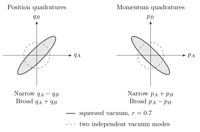
Equal-relative-height contours of the joint $q_A,q_B$ distribution (left) and the joint $p_A,p_B$ distribution (right), for $r=0.7$. Each ellipse has principal standard deviations $e^{\pm r}/\sqrt2$; the dashed circles show independent vacua. These are two separate measurement settings, not simultaneous values assigned to all four quadratures. Both panels have the same scale.

Relation to the EPR Argument and Bell Theorem

The state language here is the input to several deeper questions:

• The EPR argument asks what perfect remote predictability should imply about physical reality and completeness.
• Bell’s theorem shows that broad classes of local hidden-variable explanations cannot reproduce all quantum correlations.
• Modern continuous-variable experiments use finite squeezing, loss models, detector efficiencies, and statistical inequalities rather than the literal ideal state.

Those questions require measurement assumptions and locality assumptions beyond this page. The closest discrete-state analogue in this volume is the Bell States page, which treats maximally entangled two-qubit states as states rather than as the full Bell-theorem story.

The safe rule is: use “EPR state” for the idealized continuous-variable correlation pattern, and use “EPR argument” or “Bell theorem” only when the measurement and locality claims are explicitly under discussion.

A separability bound for the joint spreads

Use dimensionless quadratures with $[q_j,p_k]=i\delta_{jk}$. For a product state with finite second moments,

$$\operatorname{Var}(q_A-q_B)+\operatorname{Var}(p_A+p_B) =\sum_{j=A,B}[\operatorname{Var}(q_j)+\operatorname{Var}(p_j)]\ge2.$$

Each mode contributes at least one by the uncertainty relation and the arithmetic–geometric mean inequality. Mixing product states cannot reduce the variance below the average within-component variance; fluctuations of the component means add a nonnegative contribution. Thus every separable state obeys the same bound. The two-mode squeezed vacuum gives $2e^{-2r}<2$ for every $r>0$, proving entanglement without assuming Gaussianity for the separable alternative.

The collective variables commute, so their small spreads violate no Heisenberg relation. Their conjugates are the complementary combinations $q_A+q_B$ and $p_A-p_B$, whose variances grow as $e^{2r}$. This separability test is not by itself a Bell test or an EPR-steering criterion; those address different assumptions about measurement outcomes and remote prediction.

References

• S. L. Braunstein and P. van Loock, “Quantum information with continuous variables,” Reviews of Modern Physics 77, 513–577 (2005), doi:10.1103/RevModPhys.77.513.
• L.-M. Duan, G. Giedke, J. I. Cirac, and P. Zoller, “Inseparability criterion for continuous variable systems,” Physical Review Letters 84, 2722–2725 (2000), doi:10.1103/PhysRevLett.84.2722.
• A. Einstein, B. Podolsky, and N. Rosen, “Can quantum-mechanical description of physical reality be considered complete?,” Physical Review 47, 777–780 (1935), doi:10.1103/PhysRev.47.777.
• M. D. Reid, P. D. Drummond, W. P. Bowen, E. G. Cavalcanti, P. K. Lam, H. A. Bachor, U. L. Andersen, and G. Leuchs, “Colloquium: The Einstein–Podolsky–Rosen paradox: From concepts to applications,” Reviews of Modern Physics 81, 1727–1751 (2009), doi:10.1103/RevModPhys.81.1727.

Exercises

1. Commuting collective observables. Verify that $X_1-X_2$ commutes with $P_1+P_2$.

Solution

Use $[X_i,P_j]=i\hbar\delta_{ij}$ and operators on different particles commuting:

$$\begin{aligned} [X_1-X_2,P_1+P_2] &= [X_1,P_1]+[X_1,P_2] -[X_2,P_1]-[X_2,P_2] \\ &= i\hbar+0-0-i\hbar \\ &= 0. \end{aligned}$$

2. Generalized eigenfunction. Show that

$$\Psi_{x_0,P}(x_1,x_2) = \mathcal N \exp\!\left[ \frac{iP}{2\hbar}(x_1+x_2) \right] \delta(x_1-x_2-x_0)$$

is a generalized eigenfunction of $P_1+P_2$ with eigenvalue $P$.

Solution

In the position representation,

$$P_1+P_2 = -i\hbar \left( \partial_{x_1}+\partial_{x_2} \right).$$

The derivative of $\delta(x_1-x_2-x_0)$ under $\partial_{x_1}+\partial_{x_2}$ is zero because the two derivatives enter with opposite signs. Acting on the phase gives

$$-i\hbar \left( \frac{iP}{2\hbar} + \frac{iP}{2\hbar} \right) \Psi_{x_0,P} = P\Psi_{x_0,P}.$$

3. Normalizing the Gaussian approximation. For finite $\sigma,\Sigma>0$, compute $\mathcal N_{\sigma,\Sigma}$ for the Gaussian approximation in the page.

Solution

Use $r=x_1-x_2$ and $s=x_1+x_2$, with $dx_1\,dx_2=dr\,ds/2$. The squared norm is

$$\lvert\mathcal N_{\sigma,\Sigma}\rvert^2 \frac12 \int_{-\infty}^{\infty}dr\, e^{-(r-x_0)^2/(2\sigma^2)} \int_{-\infty}^{\infty}ds\, e^{-s^2/(2\Sigma^2)}.$$

The two Gaussian integrals give $\sqrt{2\pi}\sigma$ and $\sqrt{2\pi}\Sigma$, so the norm is

$$\lvert\mathcal N_{\sigma,\Sigma}\rvert^2 \pi\sigma\Sigma.$$

Setting it to one gives

$$\mathcal N_{\sigma,\Sigma} = \frac{1}{\sqrt{\pi\sigma\Sigma}},$$

up to an overall phase.

4. Finite squeezing. In the two-mode squeezed vacuum convention used on the page, what happens to $\operatorname{Var}(q_A-q_B)$, $\operatorname{Var}(p_A+p_B)$, and $\bar n$ as $r\to\infty$?

Solution

The variances are

$$\operatorname{Var}(q_A-q_B) = \operatorname{Var}(p_A+p_B) = e^{-2r},$$

so both go to zero. The mean occupation is

$$\bar n = \sinh^2 r,$$

which diverges. The ideal EPR limit therefore requires unbounded energy in this family of states.

5. A finite resource. Take $r=(\ln2)/2$. Find both EPR variances, the mean occupation per mode, and the separability-test value.

Solution

Since $e^{2r}=2$, each EPR variance is $1/2$. Also $\sinh r=(\sqrt2-1/\sqrt2)/2=1/(2\sqrt2)$, so $\bar n=1/8$. The sum of variances is one, below the separable lower bound two. Finite squeezing is sufficient to establish entanglement; no singular ideal state is required.